5. The First Law and Its Consequences

Supplement to Chapter 5 of A First Course in Atmospheric Thermodynamics by Grant W. Petty, Sundog Publishing, 2008

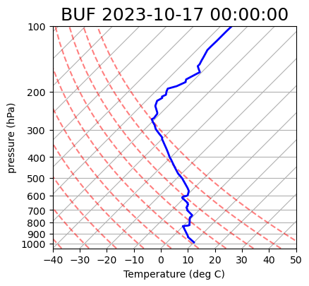
Plotting dry adiabats on a Skew-T diagram

Import necessary packages

import matplotlib.pyplot as plt
from datetime import datetime
from metpy.plots import SkewT
from siphon.simplewebservice.wyoming import WyomingUpperAir

Grab some data

date = datetime(year=2023, month=10, day=17, hour=00) # year, month, day, hour
station = 'BUF'  # station code for Buffalo, NY
df = WyomingUpperAir.request_data(date, station)

Make a plot

fig = plt.figure(figsize=(9, 9))
skew = SkewT(fig=fig, subplot=(2,1,2), rotation=45)
skew.plot(df['pressure'], df['temperature'], 
        'b', linewidth=2)
skew.ax.set_title(f'{station} {date}', fontsize=18);
skew.plot_dry_adiabats()  # some nice automation from the MetPy package here
skew.ax.set_xlabel('Temperature (deg C)')
skew.ax.set_ylabel('pressure (hPa)');