ATM350 Introductory Notebook - ATM 350, Spring 2026

This notebook displays the 54-hour forecast output from the GFS¶

import xarray as xr
import datetime as dt
import numpy as np
import pandas as pd
import matplotlib.pyplot as plt
from cartopy import crs as ccrs
from cartopy import feature as cfeature
from cartopy import util as cu
from pyproj import Proj
from metpy.units import units

Parse the current time and choose a recent hour when we might expect the model run to be complete.¶

now = dt.datetime.now()
year = now.year
month = now.month
day = now.day
hour = now.hour
print (year, month, day, hour)

if (hour >= 18):
    runHour = 12
    hr_delta = hour - runHour
elif (hour >= 12):
    runHour = 6
    hr_delta = hour - runHour
elif (hour >= 6):
    runHour = 0
    hr_delta = hour - runHour
else:
    runHour = 18
    hr_delta = hour + 6
runTime = now - dt.timedelta(hours=hr_delta)
runTimeStr = runTime.strftime('%Y%m%d %H00 UTC')
modelDate = runTime.strftime('%Y%m%d')
modelHour = runTime.strftime('%H')
modelDay = runTime.strftime('%D')

print (modelDay)
print (modelHour)
print (runTimeStr)

fhr=54
fcst_time = runTime + dt.timedelta(hours=fhr)
fcst_time = fcst_time.replace(minute = 0, second = 0, microsecond = 0)
fcst_time_str = fcst_time.strftime('%Y%m%d %H00 UTC')
print(fcst_time_str)

2026 1 22 19
01/22/26
12
20260122 1200 UTC
20260124 1800 UTC

Create an object pointing to the dataset. The GFS is available from Unidata’s THREDDS server in resolutions as high as 0.25 x 0.25 degrees! The resulting sizes of the datasets increase inversely with the magntiude of gridpont resolution.¶

URL = 'https://thredds.ucar.edu/thredds/dodsC/grib/NCEP/GFS/Global_0p25deg/GFS_Global_0p25deg_'+ modelDate + '_' + modelHour + '00.grib2'
print (URL)
ds = xr.open_dataset (URL).metpy.parse_cf()

https://thredds.ucar.edu/thredds/dodsC/grib/NCEP/GFS/Global_0p25deg/GFS_Global_0p25deg_20260122_1200.grib2

Set up objects corresponding to a few fields of interest. Our ultimate goal is to generate a map at the 850 hPa level, so we will be looking for variables on isobaric surfaces.¶

Z = ds.Geopotential_height_isobaric
T = ds.Temperature_isobaric

Subset the data and plot the figure.¶

level = 85000
latN = 52
latS = 18
cLat = (latN + latS) / 2.0
# for degrees West, add 360 so values match how they are in the dataset!
lonW = -130 + 360
lonE = -50 + 360
cLon = (lonW + lonE) / 2.0
# Create a list of values for lat and lon
expand = 10
lats = np.arange(latN + expand,latS-0.25,-0.25) # remember, latitutde go from north to south in this dataset
lons = np.arange(lonW - expand, lonE+expand+.25,0.25)

scalar0 = T.metpy.sel(lat=lats, lon=lons, time=fcst_time, vertical=level).metpy.convert_units('degC')
scalar1 = Z.metpy.sel(lat=lats, lon=lons, time=fcst_time, vertical=level).metpy.convert_units('dam')
x, y = scalar0.lon, scalar0.lat

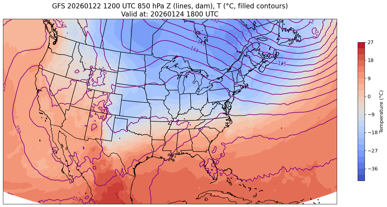
tl1 = f'GFS {runTimeStr} {level/100:.0f} hPa Z (lines, dam), T (°C, filled contours)'
tl2 = f'Valid at: {fcst_time_str}'
title_line = f"{tl1}\n{tl2}"

proj_map = ccrs.LambertConformal(central_longitude=cLon, central_latitude=cLat)
proj_data = ccrs.PlateCarree()
res = '50m'
ZCint = np.arange(99,180,3)
TCfill = np.arange (-42,30,3)
ZContourParams = dict(levels=ZCint,transform=proj_data,linewidths=1.5,colors='purple')
TContourParams = dict(levels=TCfill,transform=proj_data,cmap='coolwarm')

constrainLon = 8
fig = plt.figure(figsize=(18,12))
ax = plt.subplot(1,1,1,projection=proj_map)
ax.set_extent ([lonW + constrainLon, lonE - constrainLon, latS, latN])
ax.add_feature(cfeature.COASTLINE.with_scale(res))
ax.add_feature(cfeature.STATES.with_scale(res))
CF = ax.contourf(x,y,scalar0, **TContourParams)
cbar = plt.colorbar(CF,shrink=0.5)
cbar.ax.tick_params(labelsize=12)
cbar.ax.set_ylabel("Temperature (°C)",fontsize=12)
CL = ax.contour(x,y,scalar1, **ZContourParams)
ax.clabel(CL, inline_spacing=0.2, fontsize=11, fmt='%.0f')

title = plt.title(title_line,fontsize=16)