Meteogram - ATM 350, Spring 2026

Here we draw a surface meteogram, from data that we retrieve from our METAR archive.¶

Imports¶

import numpy as np
import pandas as pd

import matplotlib.pyplot as plt
from matplotlib.dates import DateFormatter, AutoDateLocator,YearLocator, HourLocator,DayLocator,MonthLocator

from metpy.units import units
from datetime import datetime, timedelta
import seaborn as sns

Set the desired start and end time (UTC), and create strings for the figure title.

startTime = datetime(2026,2,22,0)
endTime = datetime(2026,2,25,0)
sTimeStr = startTime.strftime(format="%x %H UTC")
eTimeStr = endTime.strftime(format="%x %H UTC")

Create an empty Dateframe to which we will concatenate the hourly CSV files in the desired time range.

df = pd.DataFrame()

Loop over each hour. Concatenate each hour’s METARs into the full Dataframe.

curTime = startTime
while (curTime <= endTime):
    print (curTime)
    timeStr = curTime.strftime("%y%m%d%H")
    metarCSV = f'/ktyle_rit/scripts/sflist2/complete/{timeStr}.csv'
    dfTemp = pd.read_csv(metarCSV, sep='\\s+')
    df = pd.concat([df, dfTemp], ignore_index=True)
    curTime = curTime + timedelta(hours=1)

2026-02-22 00:00:00
2026-02-22 01:00:00
2026-02-22 02:00:00
2026-02-22 03:00:00
2026-02-22 04:00:00
2026-02-22 05:00:00
2026-02-22 06:00:00

2026-02-22 07:00:00
2026-02-22 08:00:00
2026-02-22 09:00:00
2026-02-22 10:00:00
2026-02-22 11:00:00
2026-02-22 12:00:00

2026-02-22 13:00:00
2026-02-22 14:00:00
2026-02-22 15:00:00
2026-02-22 16:00:00
2026-02-22 17:00:00

2026-02-22 18:00:00
2026-02-22 19:00:00
2026-02-22 20:00:00
2026-02-22 21:00:00
2026-02-22 22:00:00

2026-02-22 23:00:00
2026-02-23 00:00:00
2026-02-23 01:00:00
2026-02-23 02:00:00

2026-02-23 03:00:00
2026-02-23 04:00:00
2026-02-23 05:00:00
2026-02-23 06:00:00
2026-02-23 07:00:00

2026-02-23 08:00:00
2026-02-23 09:00:00
2026-02-23 10:00:00
2026-02-23 11:00:00

2026-02-23 12:00:00
2026-02-23 13:00:00
2026-02-23 14:00:00
2026-02-23 15:00:00

2026-02-23 16:00:00
2026-02-23 17:00:00
2026-02-23 18:00:00
2026-02-23 19:00:00

2026-02-23 20:00:00
2026-02-23 21:00:00
2026-02-23 22:00:00
2026-02-23 23:00:00

2026-02-24 00:00:00
2026-02-24 01:00:00
2026-02-24 02:00:00
2026-02-24 03:00:00

2026-02-24 04:00:00
2026-02-24 05:00:00
2026-02-24 06:00:00

2026-02-24 07:00:00
2026-02-24 08:00:00
2026-02-24 09:00:00
2026-02-24 10:00:00

2026-02-24 11:00:00
2026-02-24 12:00:00
2026-02-24 13:00:00
2026-02-24 14:00:00

2026-02-24 15:00:00
2026-02-24 16:00:00
2026-02-24 17:00:00

2026-02-24 18:00:00
2026-02-24 19:00:00
2026-02-24 20:00:00

2026-02-24 21:00:00
2026-02-24 22:00:00
2026-02-24 23:00:00

2026-02-25 00:00:00

Examine the Dataframe

df

Select the station from which to subset the Dataframe.

site = 'PVD'

Create a new Dataframe that contains only the rows for the desired site.

dfSub = df.query('STN == @site')

Create a new column that represents the date and time as a datetime64 object.

# Next line suppresses a warning message. See https://pandas.pydata.org/pandas-docs/stable/user_guide/indexing.html#returning-a-view-versus-a-copy. 
# This won't be necessary with Pandas version 3 and beyond.

pd.options.mode.copy_on_write = True 

dattim = pd.to_datetime(dfSub['YYMMDD/HHMM'],format="%y%m%d/%H%M", utc=True)
dfSub['DATETIME'] = dattim

Examine the subsetted Dataframe.

dfSub

Select a couple of variables we wish to plot on the meteogram. In this case, 2m temperature and dewpoint.

var1 = dfSub['TMPC']
var2 = dfSub['DWPC']

Examine one of the variables ... of course, it’s a Pandas Series.

var1

1003      0.0
5469      0.0
9869     -0.6
14309    -0.6
18724    -0.6
         ... 
302221   -1.1
306485   -1.1
310973   -1.7
315460   -2.8
319926   -3.9
Name: TMPC, Length: 73, dtype: float64

Pandas Series objects don’t support units. We can, however, create Numpy arrays from the Series values attribute and then attach units to them.

tmpc = var1.values * units('degC')
dwpc = var2.values * units('degC')

Examine one of the units-aware arrays.

tmpc

Now convert into degrees F.

tmpf = tmpc.to('degF')
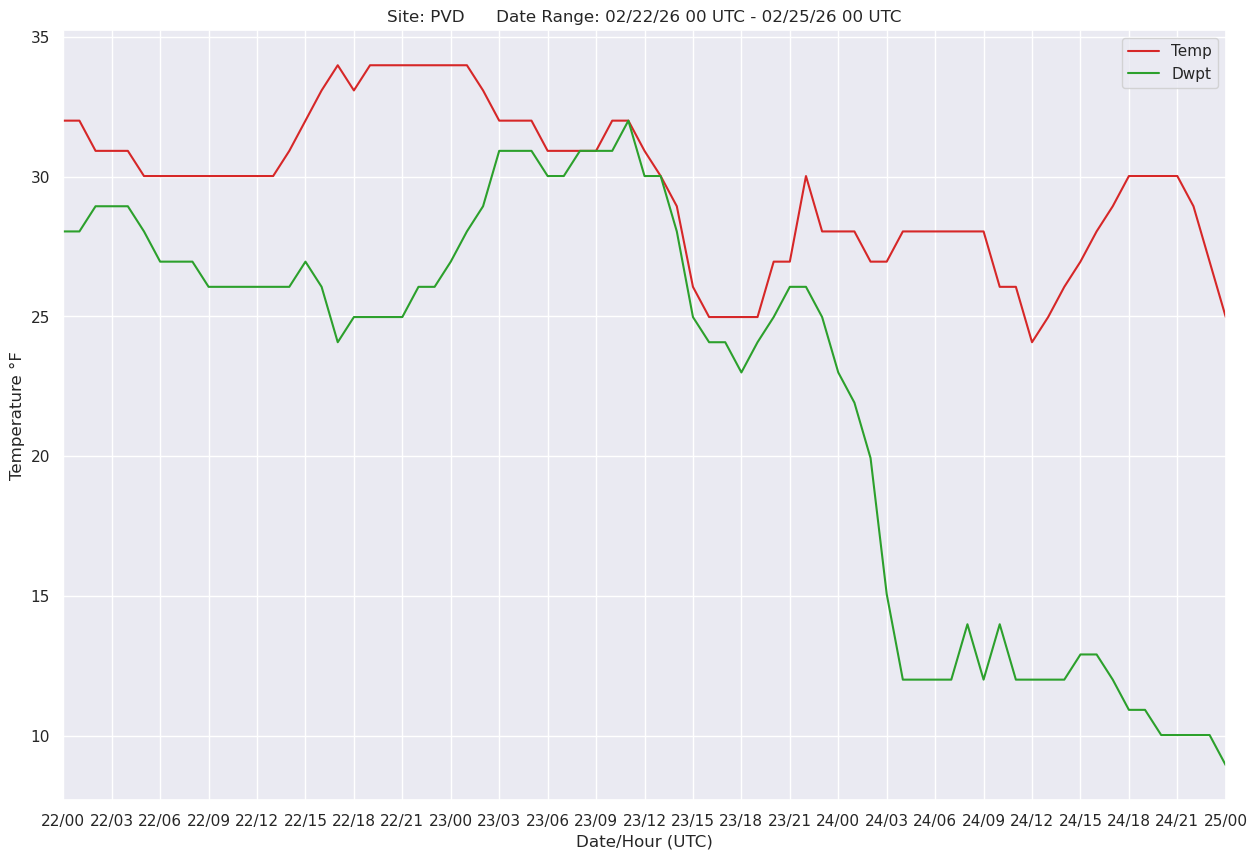
dwpf = dwpc.to('degF')

Create the meteogram and save the figure to disk.¶

sns.set()

fig, ax = plt.subplots(figsize=(15, 10))

# Improve on the default ticking

ax.xaxis.set_major_locator(HourLocator(interval=3))
hoursFmt = DateFormatter('%d/%H')
ax.xaxis.set_major_formatter(hoursFmt)

ax.plot(dfSub['DATETIME'], tmpf, color='tab:red', label='Temp')
ax.plot(dfSub['DATETIME'], dwpf, color='tab:green', label='Dwpt')

ax.set_title(f'Site: {site}      Date Range: {sTimeStr} - {eTimeStr}')

ax.set_xlabel('Date/Hour (UTC)')
ax.set_ylabel('Temperature °F')
ax.set_xlim(startTime, endTime)
ax.legend(loc='best')

fig.savefig (f'{site}_mgram.png')