04_Metpy_Regional_Metar_Map_Loop_Function
Objectives
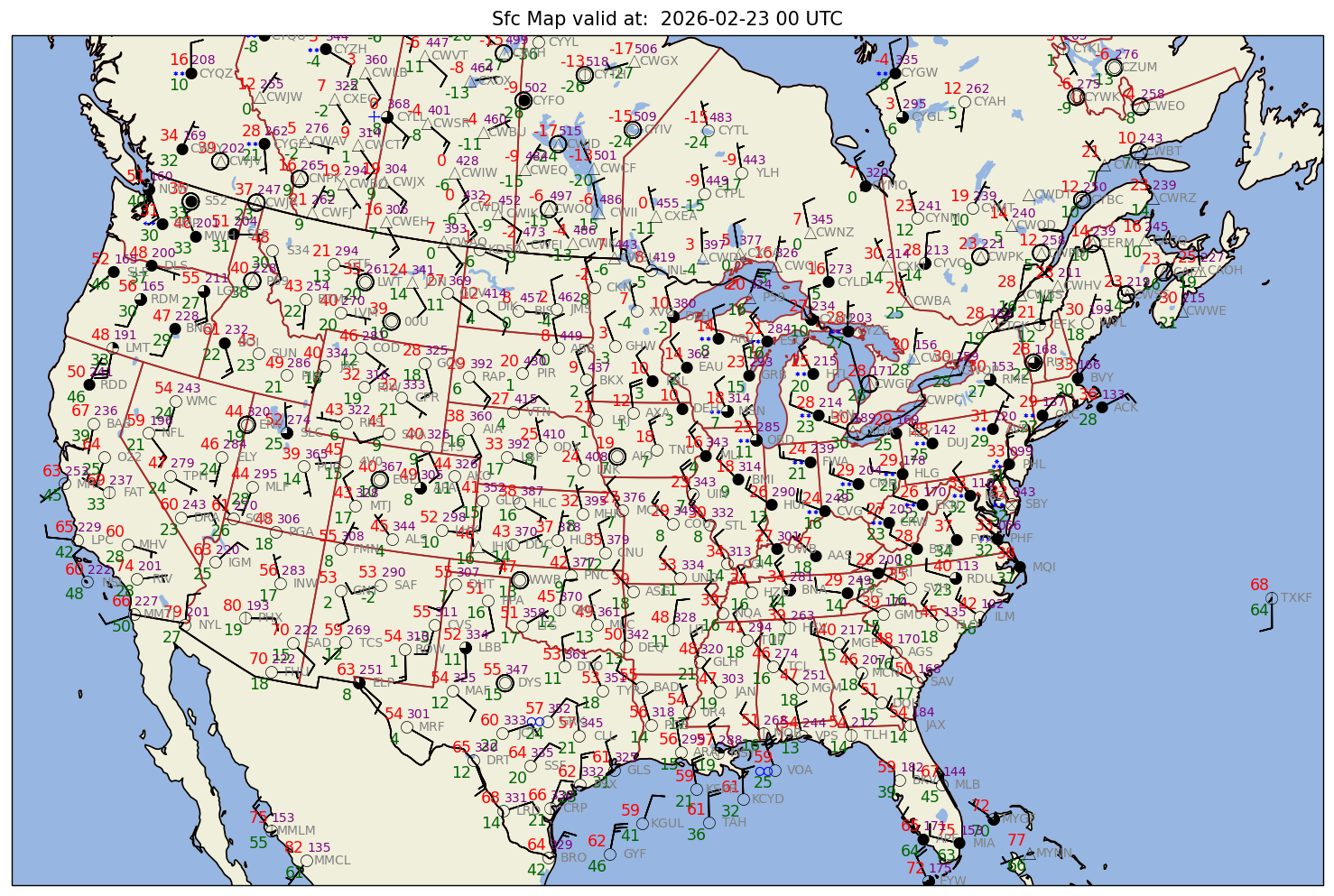
Make a surface map based on observations from worldwide METAR sites.
Modularize the Matplotlib / Cartopy customizations
Employ a loop which calls a function that does the plotting step.
Remove any text that appears outside the border of the Axes
Imports
from datetime import datetime,timedelta
from dateutil.relativedelta import relativedelta

import numpy as np
import pandas as pd
import matplotlib.pyplot as plt
import matplotlib.text as mtext

import cartopy.crs as ccrs
import cartopy.feature as cfeature

from metpy.calc import wind_components, reduce_point_density
from metpy.units import units
from metpy.plots import StationPlot, USCOUNTIES
from metpy.plots.wx_symbols import current_weather, sky_cover, wx_code_map

# Load in a collection of functions that process GEMPAK weather conditions and cloud cover data.
%run /kt11/ktyle/python/metargem.py
Determine the time range over which to gather observations.
startYear = 2026
startMonth = 2
startDay = 23
startHour = 0
startMinute = 0
startDateTime = datetime(startYear,startMonth,startDay, startHour, startMinute)

endYear = 2026
endMonth = 2
endDay = 23
endHour = 1
endMinute = 0
endDateTime = datetime(endYear,endMonth,endDay, endHour, endMinute)

delta_time = endDateTime - startDateTime
time_range_max = 7*86400

if (delta_time.total_seconds() > time_range_max):
    raise RuntimeError("Your time range must not exceed 7 days. Go back and try again.")
Create a function that handles all the common tasks involved in gathering, analyzing, and plotting surface observations for a particular time
def process_plot_metar (time_in):
    title_str = time_in.strftime("%Y-%m-%d %H UTC")
    fig_str = time_in.strftime("%Y%m%d%H")
    metar_str = time_in.strftime("%y%m%d%H")
    print(f"Processing {title_str}")
    metar_file = f'/ktyle_rit/scripts/sflist2/complete/{metar_str}.csv'
    df = pd.read_csv(metar_file, sep='\\s+')

    # ----------------------------------------------------------------
    ## Mapmaking Made Easy steps

    # 1. Set the bounds of your map.
    # Set the four values in the code cell below. Test the values.
    latN = 55
    latS = 25
    lonW = -120
    lonE = -65

    if ( latN > latS ) and ( lonE > lonW):
        cLat = (latN + latS)/2
        cLon = (lonW + lonE)/2
    else:
        e = ("Northern (eastern) latitude (longitude) must be greater than southern (western). Go back and re-adjust!")
        raise ValueError(f"Error in lat/lon specification: {e}")

    # 2. Select the map projection for your figure.
    proj_map = ccrs.LambertConformal(central_latitude=cLat, central_longitude=cLon)

    # 3. Select the projection on which the dataset is based
    proj_data = ccrs.PlateCarree()

    # 4. Select the resolution of the Cartopy cartographic features, and, if desired, MetPy's county shapefiles.

    # Uncomment / comment as desired
    #res = '10m' # Most detailed, best for small regions (e.g. NYS)
    res = '50m' # Medium detail, best for medium-sized regions (e.g. CONUS)
    #res = '110m' # Least detailed, best for large/global maps

    #res_county = '5m' # Higher-res MetPy US County shapefiles
    #res_county = '20m' # Lower-res MetPy US County shapefiles

    # 5. **Deferred till the matplotlib section** Select which cartographic features to be displayed in the figure

    ## **END ** Mapmaking Made Easy steps
    # ----------------------------------------------------------------

    ## Dataset subsetting section

    # Extend the data region beyond the plotted region

    extend = 3 # Change as necessary
    df2 = df.query('SLAT >= (@latS - @extend) & SLAT <= (@latN + @extend) & SLON  >= (@lonW - @extend) & SLON <= (@lonE + @extend)')

    # Select the weather variables of interest. Also include the site ID, lat, lon, elevation, and time columns.

    columnSubset = ['STN', 'YYMMDD/HHMM', 'SLAT', 'SLON', 'SELV', 'TMPC', 'DWPC', 'PMSL',
                'SKNT', 'DRCT','ALTI','WNUM','VSBY','CHC1', 'CHC2', 'CHC3','CTYH', 'CTYM', 'CTYL']
    df3 = df2[columnSubset]

    # ----------------------------------------------------------------

    ## Dataset value manipulation section

    # In these datasets, -9999.0 signfies missing values. Replace all instances of -9999.0 with NumPy's `NaN` (not a number) value.

    df4 = df3.replace([-9999.0, '-9999.00','********'], np.nan)
    data = df4

    # In our current data archive, multiple weather types are often not represented properly. To avoid a type conversion error, set stations whose weather type fall into this category to a missing value.

    data.loc[data['WNUM'] =='********', ['WNUM']] = '-9999.00'
    data['WNUM'] = data['WNUM'].astype('float16')

    # ----------------------------------------------------------------

    ## Meteorological parameter definition, calculation, and units assignment/conversion section
    # Read in several of the columns as Pandas `Series`; extract the value arrays from the `Series` objects; assign / convert units as necessary; convert GEMPAK cloud cover and present wx symbols to MetPy's representation

    lats = data['SLAT'].values
    lons = data['SLON'].values
    tair = (data['TMPC'].values * units ('degC')).to('degF')
    dewp = (data['DWPC'].values * units ('degC')).to('degF')
    altm = (data['ALTI'].values * units('inHg')).to('mbar')
    slp = data['PMSL'].values * units('hPa')

    # Convert wind to components
    u, v = wind_components(data['SKNT'].values * units.knots, data['DRCT'].values * units.degree)

    # replace missing wx codes or those >= 100 with 0, and convert to MetPy's present weather code
    wnum = (np.nan_to_num(data['WNUM'].values,True).astype(int))
    convert_wnum (wnum)

    # Need to handle missing (NaN) and convert to proper code
    chc1 = (np.nan_to_num(data['CHC1'].values,True).astype(int))
    chc2 = (np.nan_to_num(data['CHC2'].values,True).astype(int))
    chc3 = (np.nan_to_num(data['CHC3'].values,True).astype(int))
    cloud_cover = calc_clouds(chc1, chc2, chc3)

    # Set a variable to be used for plotting the station ID's
    stid = data['STN']

    # ----------------------------------------------------------------

    ## Station filtering section

    # Adjust point density so that there's only one point within a circle whose distance is specified in meters.
    # This value will need to change depending on how large of an area you are plotting!


    spacing = 150000 # meters; change depending on the map area, figure size, and text font size
    xy = proj_map.transform_points(proj_data, lons, lats)
    mask = reduce_point_density(xy, spacing)

    # ----------------------------------------------------------------

    ## Figure plotting section

    # First set dpi ("dots per inch") - higher values will give us a less pixelated final figure. Default is 100.
    dpi = 125

    # Set figure size. Default is 11x8.5
    fig = plt.figure(figsize=(15, 12), dpi=dpi)

    # Mapmaking Made Easy Step 2
    ax = fig.add_subplot(1, 1, 1, projection=proj_map)

    # Mapmaking Made Easy Step 1

    ax.set_extent ((lonW, lonE, latS, latN ), crs=ccrs.PlateCarree())

    # Cartographic feature selection (Mapmaking Made Easy Step 5)
    ax.set_facecolor(cfeature.COLORS['water'])
    land_mask = cfeature.NaturalEarthFeature('physical', 'land', res,
                                        edgecolor='face',
                                        facecolor=cfeature.COLORS['land'])
    lake_mask = cfeature.NaturalEarthFeature('physical', 'lakes', res,
                                        edgecolor='face',
                                        facecolor=cfeature.COLORS['water'])
    state_borders = cfeature.NaturalEarthFeature(category='cultural', name='admin_1_states_provinces_lakes',
                                         scale=res, facecolor='none')

    country_borders = cfeature.NaturalEarthFeature(category='cultural', name='admin_0_countries',
                                         scale=res, facecolor='none')

    ax.add_feature(land_mask)
    ax.add_feature(lake_mask)
    ax.add_feature(state_borders, linestyle='solid', edgecolor='brown')
    ax.add_feature(country_borders, linestyle='solid', edgecolor='black')

    # Uncomment if we wanted to add county borders to our plot:
    #ax.add_feature(USCOUNTIES.with_scale(res_county), linewidth=0.8, edgecolor='darkgray')

    #Uncomment if we wanted to add grid lines to our plot:
    #ax.gridlines()

    # Create a station plot pointing to an Axes to draw on as well as the location of points
    stationplot = StationPlot(ax, lons[mask], lats[mask], transform=proj_data,
                          fontsize=8)
    stationplot.plot_parameter('NW', tair[mask], color='red', fontsize=10)
    stationplot.plot_parameter('SW', dewp[mask], color='darkgreen', fontsize=10)

    # Below, we are using a custom formatter to control how the sea-level pressure values are plotted.
    # This uses the standard trailing 3-digits of the pressure value in tenths of millibars.
    stationplot.plot_parameter('NE', slp[mask], color='purple', formatter=lambda v: format(10 * v, '.0f')[-3:])

    stationplot.plot_symbol('C', cloud_cover[mask], sky_cover)
    stationplot.plot_symbol('W', wnum[mask], current_weather,color='blue',fontsize=12)
    stationplot.plot_text((2, 0),stid[mask], color='gray')

    #zorder - Higher value zorder will plot the variable on top of lower value zorder. This is necessary for wind barbs to appear. Default is 1.
    stationplot.plot_barb(u[mask], v[mask],zorder=2)

    plotTitle = (f"Sfc Map valid at:  {title_str}")
    ax.set_title (plotTitle)

    # Remove any text that appears outside the borders of the Axes

    for obj in ax.findobj(mtext.Text):
        obj.set_clip_on(True)

    # Write out graphic to disk
    region = 'CONUS' # e.g., 'CONUS', 'NYS', 'Caribbean', etc.
    figName = (f'{fig_str}_{region}_sfmap.png')
    fig.savefig(figName);
Set the initial time, the time interval, and then call the function defined above.
time_incr = relativedelta(hours=1)
valid_time = startDateTime

while (valid_time < endDateTime):

    process_plot_metar(valid_time)

    valid_time = valid_time + time_incr
Processing 2026-02-23 00 UTC
/tmp/ipykernel_1591192/201419437.py:71: FutureWarning: Setting an item of incompatible dtype is deprecated and will raise an error in a future version of pandas. Value '-9999.00' has dtype incompatible with float64, please explicitly cast to a compatible dtype first.
  data.loc[data['WNUM'] =='********', ['WNUM']] = '-9999.00'
Next steps
To further modularize this workflow, we would seek to divide the single function above into multiple functions. These might include:
Opening the data file
Subset and perform calculations/unit conversions
Define attributes of the plot and map