Pandas 3: Plotting NYS Mesonet Observations¶

Overview¶

In this notebook, we’ll use Pandas to read in and analyze current data from the New York State Mesonet. We will also use Matplotlib to plot the locations of NYSM sites.

Prerequisites¶

Concepts	Importance	Notes
Matplotlib	Necessary
Pandas	Necessary

Time to learn: 15 minutes

Imports¶

import matplotlib.pyplot as plt
import numpy as np
import pandas as pd

Create a Pandas DataFrame object pointing to the latest set of obs.

nysm_data = pd.read_csv('https://www.atmos.albany.edu/products/nysm/nysm_latest.csv')

nysm_data

Loading...

Create Series objects for several columns from the DataFrame.

First, remind ourselves of the column names.

nysm_data.columns

Index(['station', 'time', 'temp_2m [degC]', 'temp_9m [degC]',
       'relative_humidity [percent]', 'precip_incremental [mm]',
       'precip_local [mm]', 'precip_max_intensity [mm/min]',
       'avg_wind_speed_prop [m/s]', 'max_wind_speed_prop [m/s]',
       'wind_speed_stddev_prop [m/s]', 'wind_direction_prop [degrees]',
       'wind_direction_stddev_prop [degrees]', 'avg_wind_speed_sonic [m/s]',
       'max_wind_speed_sonic [m/s]', 'wind_speed_stddev_sonic [m/s]',
       'wind_direction_sonic [degrees]',
       'wind_direction_stddev_sonic [degrees]', 'solar_insolation [W/m^2]',
       'station_pressure [mbar]', 'snow_depth [cm]', 'frozen_soil_05cm [bit]',
       'frozen_soil_25cm [bit]', 'frozen_soil_50cm [bit]',
       'soil_temp_05cm [degC]', 'soil_temp_25cm [degC]',
       'soil_temp_50cm [degC]', 'soil_moisture_05cm [m^3/m^3]',
       'soil_moisture_25cm [m^3/m^3]', 'soil_moisture_50cm [m^3/m^3]', 'lat',
       'lon', 'elevation', 'name'],
      dtype='object')

Create several Series objects for particular columns of interest.

stid = nysm_data['station']
lats = nysm_data['lat']
lons = nysm_data['lon']
time = nysm_data['time']
tmpc = nysm_data['temp_2m [degC]']
tmpc9 = nysm_data['temp_9m [degC]']
rh   = nysm_data['relative_humidity [percent]']
pres = nysm_data['station_pressure [mbar]']
wspd = nysm_data['max_wind_speed_prop [m/s]']
drct = nysm_data['wind_direction_prop [degrees]']
pinc = nysm_data['precip_incremental [mm]']
ptot = nysm_data['precip_local [mm]']
pint = nysm_data['precip_max_intensity [mm/min]']

time

0      2026-03-13 00:20:00
1      2026-03-13 00:20:00
2      2026-03-13 00:20:00
3      2026-03-13 00:20:00
4      2026-03-13 00:20:00
              ...         
122    2026-03-13 00:20:00
123    2026-03-13 00:20:00
124    2026-03-13 00:20:00
125    2026-03-13 00:20:00
126    2026-03-13 00:20:00
Name: time, Length: 127, dtype: object

Examine one or more of these Series.

tmpc

0     -2.3
1     -2.0
2     -1.7
3      2.6
4     -2.7
      ... 
122   -6.4
123   -3.0
124    0.2
125   -0.6
126   -0.3
Name: temp_2m [degC], Length: 127, dtype: float64

# Write your code below

Convert the temperature and wind speed arrays to Fahrenheit and knots, respectively.

tmpf = tmpc * 1.8 + 32
wspk = wspd * 1.94384

Examine the new Series. Note that every element of the array has been calculated using the arithemtic above ... in just one line of code per Series!

tmpf

0      27.86
1      28.40
2      28.94
3      36.68
4      27.14
       ...  
122    20.48
123    26.60
124    32.36
125    30.92
126    31.46
Name: temp_2m [degC], Length: 127, dtype: float64

tmpf.name = 'temp_2m [degF]'

tmpf

0      27.86
1      28.40
2      28.94
3      36.68
4      27.14
       ...  
122    20.48
123    26.60
124    32.36
125    30.92
126    31.46
Name: temp_2m [degF], Length: 127, dtype: float64

Next, get the basic statistical properties of one of the Series.

tmpf.describe()

count    127.000000
mean      29.368031
std        3.666102
min       20.480000
25%       26.960000
50%       29.660000
75%       31.820000
max       40.280000
Name: temp_2m [degF], dtype: float64

tmpc9

0     -2.2
1     -2.4
2     -1.4
3      2.4
4     -2.7
      ... 
122   -6.6
123   -2.9
124    0.4
125   -0.6
126   -0.4
Name: temp_9m [degC], Length: 127, dtype: float64

Check if any of the values are set to missing (NaN, aka Not-a-Number)

missing = tmpc9.isna()

missing

0      False
1      False
2      False
3      False
4      False
       ...  
122    False
123    False
124    False
125    False
126    False
Name: temp_9m [degC], Length: 127, dtype: bool

nysm_data[missing]

Loading...

# Write your code below

Plot station locations using Matplotlib¶

We use another plotting method for an Axes element ... in this case, a Scatter plot. We pass as arguments into this method the x- and y-arrays, corresponding to longitudes and latitudes, and then set five additional attributes.

fig = plt.figure(figsize=(12,9))
ax = fig.add_subplot(1,1,1)
ax.set_title ('New York State Mesonet Site Locations')
ax.scatter(lons,lats,s=9,c='r',edgecolor='black',alpha=0.75)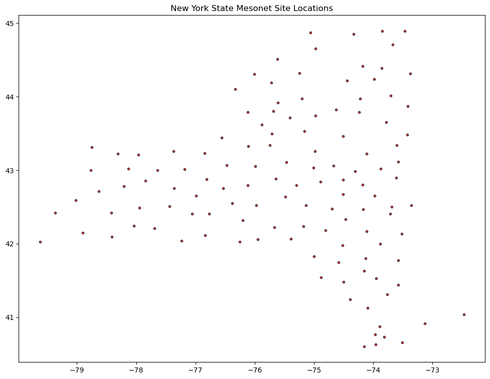

# Write your code below

What’s Next?¶

We can discern the outline of New York State! But wouldn’t it be nice if we could plot cartographic features, such as physical and/or political borders (e.g., coastlines, national/state/provincial boundaries), as well as georeference the data we are plotting? We’ll cover that next with the Cartopy package!