HW3_Q2_Metpy_METAR_NYSM: Example Solution
Objectives
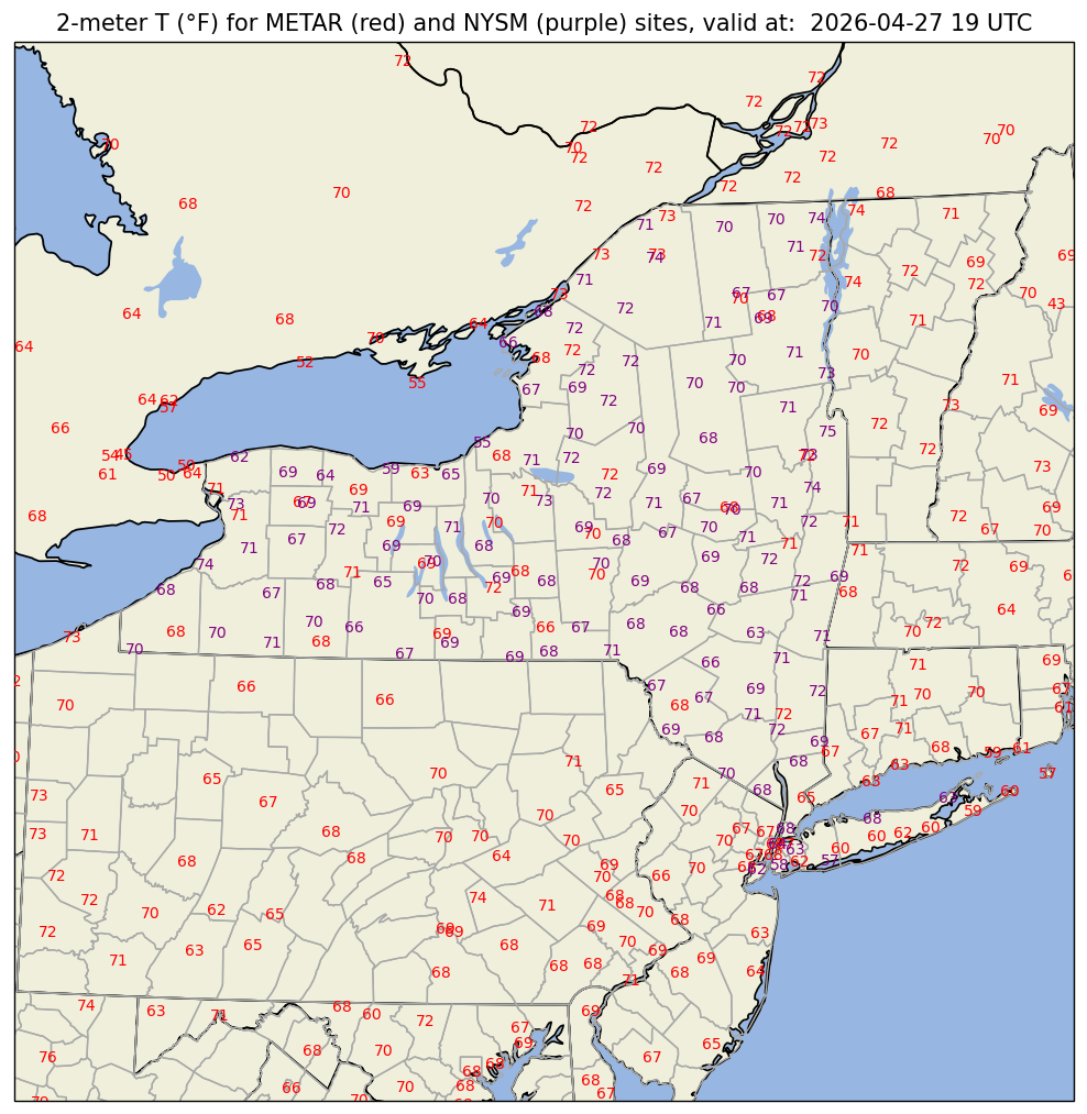
Overlay current NYSM and METAR temperatures on a map centered over New York State.
Imports
from datetime import datetime,timedelta
import numpy as np
import pandas as pd
import matplotlib.pyplot as plt
import matplotlib.text as mtext

import cartopy.crs as ccrs
import cartopy.feature as cfeature

from metpy.calc import reduce_point_density
from metpy.units import units
from metpy.plots import StationPlot, USCOUNTIES# Use the current time, or set your own for a past time.
# Set current to False if you want to specify a past time
current = True
#current = False
if (current):
validTime = datetime.now()
year = validTime.year
month = validTime.month
day = validTime.day
hour = validTime.hour
minute = validTime.minute
validTime = datetime(year, month, day, hour, minute)
offset = timedelta(minutes = 10)
validTime = validTime - offset
else:
year = 2024
month = 9
day = 26
hour = 18
minute = 0
validTime = datetime(year, month, day, hour, minute)
timeStr = validTime.strftime("%Y-%m-%d %H UTC")
timeStr2 = validTime.strftime("%Y%m%d%H")
YYMMDDHH = validTime.strftime("%y%m%d%H")
print(timeStr)
print(validTime)2026-04-27 19 UTC
2026-04-27 19:32:00
Open the hourly METAR file
metarFile = f'/ktyle_rit/scripts/sflist2/complete/{YYMMDDHH}.csv'
dfM = pd.read_csv(metarFile, sep='\\s+')
dfM
Loading...
Read in the latest set of NYSM obs.
dfN = pd.read_csv('https://www.atmos.albany.edu/products/nysm/nysm_latest.csv')Extract 2m temperature, lat, and lon from the NYSM dataframe
t2m_nysm = (dfN['temp_2m [degC]'].values * units('degC')).to('degF')
lat_nysm = dfN['lat'].values
lon_nysm = dfN['lon'].values
Mapmaking made easy! Follow these steps:
1. Set the bounds of your map.
# Set the four values in the code cell below. Test the values.
latN = 45
latS = 40
lonW = -80
lonE = -72

if ( latN > latS ) and ( lonE > lonW):
    cLat = (latN + latS)/2
    cLon = (lonW + lonE)/2
else:
   e = ("Northern (eastern) latitude (longitude) must be greater than southern (western). Go back and re-adjust!")
   raise ValueError(f"Error in lat/lon specification: {e}")
2. Select the projection (i.e. Cartopy’s coordinate reference system, aka CRS) for your map.
proj_map = ccrs.LambertConformal(central_latitude=cLat, central_longitude=cLon)3. Select the projection / CRS that is valid for the dataset you are plotting
proj_data = ccrs.PlateCarree()4. Select the resolution of the Cartopy Natural Earth cartographic features, and, if desired, MetPy’s county shapefiles.
# Uncomment / comment as desired
res = '10m' # Most detailed, best for small regions (e.g. NYS)
#res = '50m' # Medium detail, best for medium-sized regions (e.g. CONUS)
#res = '110m' # Least detailed, best for large/global maps

res_county = '5m' # Use with MetPy's US County shapefiles
5. Select the cartographic features (e.g., physical ones such as coastlines or rivers, and political features like states / provinces or (national) borders) you will include in your maps.
Perform the spatial subset.
extend = 1.0 # Change as necessary
df2 = dfM.query('SLAT >= (@latS - @extend) & SLAT <= (@latN + @extend) & SLON  >= (@lonW - @extend) & SLON <= (@lonE + @extend)')
df2
Loading...
Select the weather variables of interest. Also include the site ID, lat, lon, elevation, and time columns.
columnSubset = ['STN', 'YYMMDD/HHMM', 'SLAT', 'SLON', 'SELV', 'TMPC']
df3 = df2[columnSubset]
df3
Loading...
In these datasets, -9999.0 signfies missing values. Replace all instances of -9999.0 with NumPy’s NaN (not a number) value.
df4 = df3.replace([-9999.0, '-9999.00','********'], np.nan)
data = df4
Read in the latitude, longitude, and temperature columns as Pandas Series; extract the value arrays from the Series objects; assign / convert units as necessary
lats = data['SLAT'].values
lons = data['SLON'].values
tair = (data['TMPC'].values * units ('degC')).to('degF')
In this case, we don’t want to omit any points, regardless of how close they are to each other.
spacing = 0 # meters; change depending on the map area
xy = proj_map.transform_points(proj_data, lons, lats)
mask = reduce_point_density(xy, spacing)
Plot the data on a map
Note we will need to be create two separate MetPy StationPlot instances: one for the METAR sites; the other for the NYSM sites. Otherwise, the lats/lons will not be correct for the second set of observations (in this case, the NYSM ones).
# Set up a plot with map features
# First set dpi ("dots per inch") - higher values will give us a less pixelated final figure. Default is 100.
dpi = 125

# Set figure size. Default is 11x8.5
fig = plt.figure(figsize=(15, 10), dpi=dpi)

# Mapmaking Made Easy Step 2
ax = fig.add_subplot(1, 1, 1, projection=proj_map)

# Mapmaking Made Easy Step 1
# Slightly expand the extent of the map as compared to the subsetted data region; this helps eliminate data from being plotted beyond the frame of the map
w_ext = -0.5
e_ext = 0.5
s_ext = -1
n_ext = 1
ax.set_extent ((lonW + w_ext,lonE + e_ext,latS + s_ext, latN + n_ext), crs=proj_data)

# Cartographic feature selection (Mapmaking Made Easy Step 5)
ax.set_facecolor(cfeature.COLORS['water'])
land_mask = cfeature.NaturalEarthFeature('physical', 'land', res,
                                        edgecolor='face',
                                        facecolor=cfeature.COLORS['land'])
lake_mask = cfeature.NaturalEarthFeature('physical', 'lakes', res,
                                        edgecolor='face',
                                        facecolor=cfeature.COLORS['water'])
state_borders = cfeature.NaturalEarthFeature(category='cultural', name='admin_1_states_provinces_lakes',
                                         scale=res, facecolor='none')

ax.add_feature(land_mask)
ax.add_feature(lake_mask)
ax.add_feature(state_borders, linestyle='solid', edgecolor='black')

ax.add_feature(USCOUNTIES.with_scale(res_county), linewidth=0.8, edgecolor='darkgray') # uncomment if desired!


#If we wanted to add grid lines to our plot:
#ax.gridlines()

# Create a station plot pointing to an Axes to draw on as well as the location of points
# First stationplot instance: METAR sites
stationplot = StationPlot(ax, lons[mask], lats[mask], transform=proj_data,
                          fontsize=8)

stationplot.plot_parameter('C', tair[mask], color='red', fontsize=8)


# Create a second stationplot instaance, this time for the NYSM sites.

stationplot2 = StationPlot(ax, lon_nysm, lat_nysm, transform=proj_data,
                          fontsize=8)

stationplot2.plot_parameter('C', t2m_nysm, color='purple', fontsize=8)

# Remove any text that appears outside the borders of the Axes

for obj in ax.findobj(mtext.Text):
    obj.set_clip_on(True)
plotTitle = (f"2-meter T (°F) for METAR (red) and NYSM (purple) sites, valid at:  {timeStr}")

ax.set_title (plotTitle);

# Save figure to disk
figName = (f'2mT_Combined_{timeStr2}.png')
fig.savefig(figName)