Intro to Xarray

Outline¶

Introduction to Xarray
Anatomy of a DataArray

Imports¶

import xarray as xr

While Pandas is great for many purposes, extending its inherently 2-d data representation to a multidimensional dataset, such as 4-dimensional (time, vertical level, longitude (x) and latitude (y)) gridded NWP/Climate model output, is unwise.¶

Gridded data is typically written in a non-ASCII (i.e., not human-readable) format. The two most widely-used formats are GRIB and NetCDF. Another format, quickly gaining traction, is Zarr. These binary formats take up less storage space than text.¶

The Xarray package is ideally-suited for gridded data, in particular NetCDF and Zarr. It builds and extends on the multi-dimensional data structure in NumPy. We will see that some of the same methods we’ve used for Pandas have analogues in Xarray.¶

As a a general introduction to Xarray, below is part of a section from the Xarray Tutorial that was presented at the SciPy 2020 conference:¶

(Start of SciPy 2020 Xarray Tutorial snippet)

Multi-dimensional (a.k.a. N-dimensional, ND) arrays (sometimes called “tensors”) are an essential part of computational science. They are encountered in a wide range of fields, including physics, astronomy, geoscience, bioinformatics, engineering, finance, and deep learning. In Python, NumPy provides the fundamental data structure and API for working with raw ND arrays. However, real-world datasets are usually more than just raw numbers; they have labels which encode information about how the array values map to locations in space, time, etc.

Here is an example of how we might structure a dataset for a weather forecast:

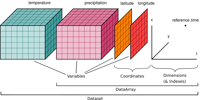
You’ll notice multiple data variables (temperature, precipitation), coordinate variables (latitude, longitude), and dimensions (x, y, t). We’ll cover how these fit into Xarray’s data structures below.

Xarray doesn’t just keep track of labels on arrays – it uses them to provide a powerful and concise interface, with methods that look a lot like Pandas. For example:

Apply operations over dimensions by name: x.sum('time').
Select values by label (or logical location) instead of integer location: x.loc['2014-01-01'] or x.sel(time='2014-01-01').
Mathematical operations (e.g., x - y) vectorize across multiple dimensions (array broadcasting) based on dimension names, not shape.
Easily use the split-apply-combine paradigm with groupby: x.groupby('time.dayofyear').mean().
Database-like alignment based on coordinate labels that smoothly handles missing values: x, y = xr.align(x, y, join='outer').
Keep track of arbitrary metadata in the form of a Python dictionary: x.attrs.

The N-dimensional nature of xarray’s data structures makes it suitable for dealing with multi-dimensional scientific data, and its use of dimension names instead of axis labels (dim='time' instead of axis=0 or axis='columns') makes such arrays much more manageable than the raw numpy ndarray: with xarray, you don’t need to keep track of the order of an array’s dimensions or insert dummy dimensions of size 1 to align arrays (e.g., using np.newaxis).

The immediate payoff of using xarray is that you’ll write less code. The long-term payoff is that you’ll understand what you were thinking when you come back to look at it weeks or months later.

(End of SciPy 2020 Xarray Tutorial snippet)

Core XArray objects: the Dataset and the DataArray¶

As did Pandas with its `Series` and `DataFrame` core data structures, Xarray also has two “workhorses”: the `DataArray` and the `Dataset`. Just as a Pandas `DataFrame` consists of multiple `Series`, an Xarray `Dataset` is made up of one or more `DataArray` objects. Let’s first look at a `Dataset`, that is Xarray’s representation of an ERA5 gridded data file.¶

# Similar to a Pandas DataFrame, we get a nice (and even more interactive) HTML representation of the object.
ds = xr.open_dataset(f'/spare11/atm350/data/199303_era5.nc')
ds

The `ds` Dataset has the following properties:¶

It has four named dimensions, in order: time, latitude, level, longitude, and level.
It has four coordinate variables, which (in this case, but not always) correspond to the dimensions.
It contains two data variable named geopotential and mean_sea_level_pressure. The data variable can be read in as a Data Array.
It has attributes which are the dataset’s metadata.
Its coordinate variables may have their own metadata as well.

DataArrays¶

When we analyze and display information in a gridded Xarray Dataset, we are actually working with one or more DataArrays within one or more Datasets. In the ERA5 dataset, there exist two gridded fields, one of whichis mean_sea_level_pressure. Let’s read it in as an Xarray DataArray object. You will see that we access it in a similar manner to how we accessed a column, aka Series, in a Pandas Dataframe.

slp = ds['mean_sea_level_pressure']

slp

Similar to (but not exactly the same as) the `ds` Dataset which contains it, this `DataArray` has the following properties:¶

It is a named data variable: mean_sea_level_pressure
It has three named dimensions, in order: time, latitude, longitude.
It has three coordinate variables, which (in this case, but not always) correspond to the dimensions.
It has attributes which are the data variable’s metadata.
Its coordinate variables may have their own metadata as well.

Let’s examine each of these five properties.¶

1. The data variable is represented by the `DataArray` object itself. We can query various properties of it, with methods similar to Pandas.¶

# Akin to column and row indices in Pandas:
slp.indexes

Indexes:
    latitude   Index([  90.0,  89.75,   89.5,  89.25,   89.0,  88.75,   88.5,  88.25,   88.0,
        87.75,
       ...
       -87.75,  -88.0, -88.25,  -88.5, -88.75,  -89.0, -89.25,  -89.5, -89.75,
        -90.0],
      dtype='float32', name='latitude', length=721)
    longitude  Index([   0.0,   0.25,    0.5,   0.75,    1.0,   1.25,    1.5,   1.75,    2.0,
         2.25,
       ...
        357.5, 357.75,  358.0, 358.25,  358.5, 358.75,  359.0, 359.25,  359.5,
       359.75],
      dtype='float32', name='longitude', length=1440)
    time       DatetimeIndex(['1993-03-01 00:00:00', '1993-03-01 06:00:00',
               '1993-03-01 12:00:00', '1993-03-01 18:00:00',
               '1993-03-02 00:00:00', '1993-03-02 06:00:00',
               '1993-03-02 12:00:00', '1993-03-02 18:00:00',
               '1993-03-03 00:00:00', '1993-03-03 06:00:00',
               ...
               '1993-03-29 12:00:00', '1993-03-29 18:00:00',
               '1993-03-30 00:00:00', '1993-03-30 06:00:00',
               '1993-03-30 12:00:00', '1993-03-30 18:00:00',
               '1993-03-31 00:00:00', '1993-03-31 06:00:00',
               '1993-03-31 12:00:00', '1993-03-31 18:00:00'],
              dtype='datetime64[ns]', name='time', length=124, freq=None)

slp.mean()

slp.max()

slp.min()

This invocation will return the lat, lon, and time of the minimum (or maximum) value in the DataArray (source: https://stackoverflow.com/questions/40179593/how-to-get-the-coordinates-of-the-maximum-in-xarray)

slp.where(slp==slp.min(),drop=True).coords

Coordinates:
  * time       (time) datetime64[ns] 8B 1993-03-24
  * latitude   (latitude) float32 4B -64.5
  * longitude  (longitude) float32 4B 78.0

We can use loc to select via dimension values, but note that order of indices must follow dimension order.

slp.loc['1993-03-14-18:00:00',42.75,286.25]

We can alternatively, (and preferably!) use Xarray’s sel indexing technique, where we specify the names of the dimension and the values we are selecting ... can be in any order ... and does not need to include all dimensions. In the cell below, we get the SLP values for this particular point for every time in the dataset.

slp.sel(longitude = 286.25, latitude = 42.75)

Similar to Pandas, Xarray includes a `plot` method into Matplotlib which we can use to get a quick view of the data. Here, we will construct a time series at a specific gridpoint.¶

ts = slp.sel(longitude = 286.25, latitude = 42.75)

ts.plot()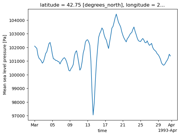

2. Dimension names¶

In Xarray, dimensions can be thought of as extensions of Pandas` 2-d row/column indices (aka axes). We can assign names, or labels, to Pandas indexes; in Xarray, these labeled axes are a necessary (and excellent) feature.

slp.dims

('time', 'latitude', 'longitude')

3. Coordinates¶

Coordinate variables in Xarray are 1-dimensional arrays that correspond to the Data variable’s dimensions. In this case, slp has dimension coordinates of longitude, latitude, and time; each of these dimension coordinates consist of an array of values, plus metadata.

slp.coords

Coordinates:
  * time       (time) datetime64[ns] 992B 1993-03-01 ... 1993-03-31T18:00:00
  * latitude   (latitude) float32 3kB 90.0 89.75 89.5 ... -89.5 -89.75 -90.0
  * longitude  (longitude) float32 6kB 0.0 0.25 0.5 0.75 ... 359.2 359.5 359.8

We can assign an object to each coordinate dimension.

lons = slp.longitude

lats = slp.latitude

time = slp.time

time

4. The data variables will typically have attributes (metadata) attached to them.¶

slp.attrs

{'long_name': 'Mean sea level pressure',
 'short_name': 'msl',
 'standard_name': 'air_pressure_at_mean_sea_level',
 'units': 'Pa'}

slp.units

'Pa'

5. The coordinate variables will likely (but not always) have metadata as well.¶

lons.attrs

{'long_name': 'longitude', 'units': 'degrees_east'}

time.attrs

{}

Create a quick plan-view data visualization at a particular time.¶

slp.sel(time='1993-03-14-18:00:00').plot(figsize=(15,10))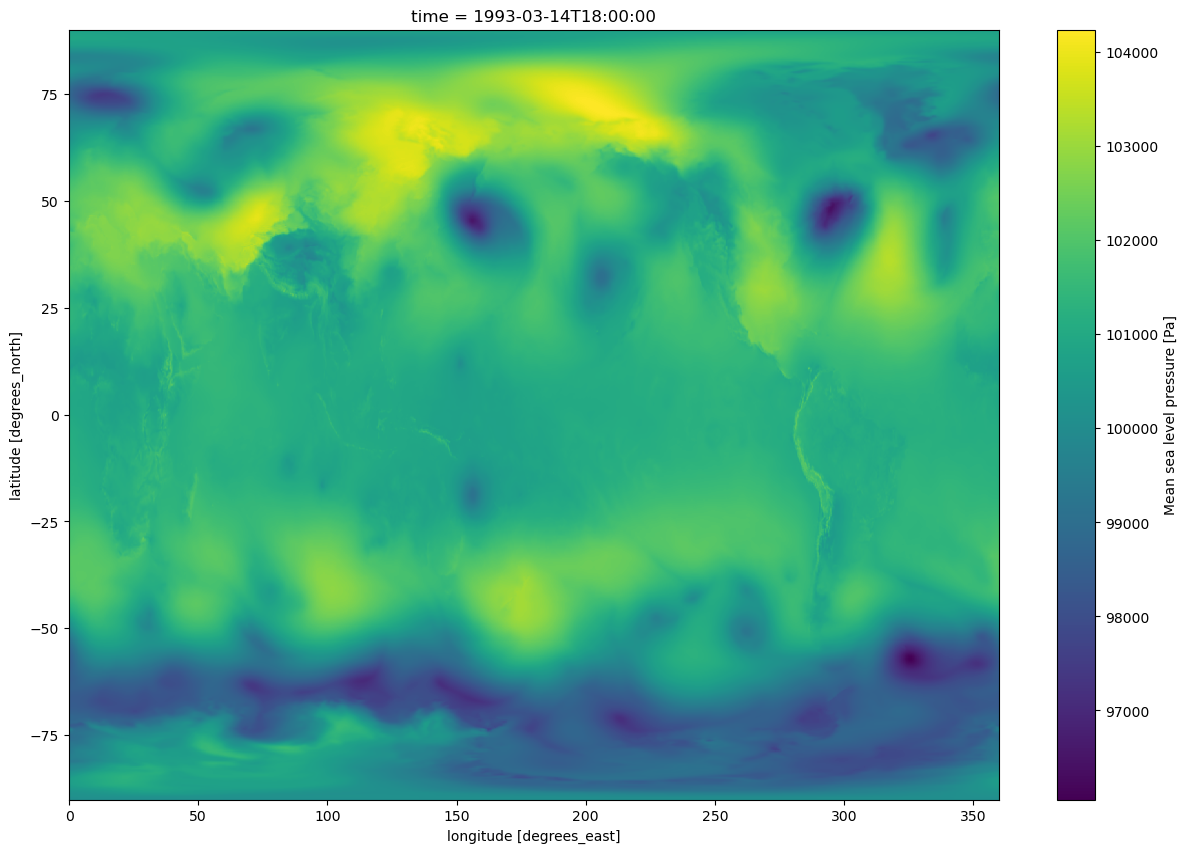

#Write your code here: