ERA5 Zarr Archive Analysis and Visualiation 1: Maps
ERA5 Zarr Archive Analysis and Visualiation 1: Maps
Overview
- Work with a cloud-served ERA5 archive
- Subset the Dataset along its dimensions
- Perform unit conversions
- Create a well-labeled multi-parameter contour plot of gridded ERA5 data
Imports
import xarray as xr
import pandas as pd
import numpy as np
from datetime import datetime as dt
from metpy.units import units
import metpy.calc as mpcalc
import cartopy.crs as ccrs
import cartopy.feature as cfeature
import matplotlib.pyplot as plt
Select the region, time, and (if applicable) vertical level(s) of interest.
# Areal extent

lonW = -100
lonE = -60
latS = 25
latN = 55
cLat, cLon = (latS + latN)/2, (lonW + lonE)/2

# Recall that in ERA5, longitudes run between 0 and 360, not -180 and 180
if (lonW < 0 ):
    lonW = lonW + 360
if (lonE < 0 ):
    lonE = lonE + 360

expand = 1
latRange = np.arange(latS - expand,latN + expand,.25) # expand the data range a bit beyond the plot range
lonRange = np.arange((lonW - expand),(lonE + expand),.25) # Need to match longitude values to those of the coordinate variable

# Vertical level specificaton
plevel = 500
levelStr = str(plevel)

# Date/Time specification
Year = 1970
Month = 1
Day = 11
Hour = 18
Minute = 0
dateTime = dt(Year,Month,Day, Hour, Minute)
timeStr = dateTime.strftime("%Y-%m-%d %H%M UTC")
Work with a cloud-served ERA5 archive
Parts of the ECMWF Reanalysis version 5 (aka ERA-5) are increasingly accessible via a Analysis Ready, Cloud Optimized (aka ARCO) format.
We will utilize Destination Earth’s Earth Data Hub (Free account required) as our primary ERA5 repository. Another one, which we will fall back on should the primary be inaccessible, is WeatherBench2.
Open an object that points to one of the two Zarr stores.
%%time
use_DE = True
#use_DE = False
if (use_DE):
  ds = xr.open_dataset(
  'https://data.earthdatahub.destine.eu/era5/reanalysis-era5-pressure-levels-v0.zarr',
  chunks={}, storage_options={"client_kwargs":{"trust_env":True}}, consolidated=True, engine="zarr"
  )

else:
    ds = xr.open_dataset(
    'gs://weatherbench2/datasets/era5/1959-2023_01_10-wb13-6h-1440x721.zarr',
     chunks = {'time':48}, consolidated = True, engine="zarr"
    )
print(f'size: {ds.nbytes / (1024 ** 4)} TB')
size: 863.9610183753794 TB
CPU times: user 1.36 s, sys: 190 ms, total: 1.55 s
Wall time: 3.89 s
The cloud-hosted datasets are big (800+TB and 40+TB) files! But Xarray is just reading only enough of the file for us to get a look at the dimensions, coordinate and data variables, and other metadata. We call this lazy loading, as opposed to eager loading, which we will do only after we have subset the dataset over time, lat-lon, and vertical level.
Examine the dataset
# Write your code here
dsData variables selection and subsetting
We’ll retrieve one variable (i.e. DataArray), geopotential, from the Dataset. Examine it after performing the subsetting.
%%time
if (use_DE):
    z = ds['z'].sel(valid_time=dateTime,isobaricInhPa=plevel,latitude=latRange,longitude=lonRange)
    t = ds['t'].sel(valid_time=dateTime,isobaricInhPa=plevel,latitude=latRange,longitude=lonRange)
else:
    z = ds['geopotential'].sel(time=dateTime,level=plevel,latitude=latRange,longitude=lonRange)
print(f'size: {z.nbytes / (1024 ** 2)} MB')
zDefine our subsetted coordinate arrays of lat and lon. Pull them from the DataArray. We’ll need to pass these into the contouring functions later on.
lats = z.latitude
lons = z.longitude
Perform unit conversions
Convert geopotential in m**2/s**2 to geopotential height in decameters (dam).
We take the DataArrays and apply MetPy’s unit conversion methods.
z = mpcalc.geopotential_to_height(z).metpy.convert_units('dam')t = t.metpy.convert_units('degC')z.nbytes / 1e3 # size in KB for the subsetted DataArrays86.016Create a well-labeled multi-parameter contour plot of gridded ERA5 reanalysis data
We will make contour fills of 500 hPa height in decameters, with a contour interval of 6 dam.
As we’ve done before, let’s first define some variables relevant to Cartopy. Recall that we already defined the areal extent up above when we did the data subsetting.
proj_map = ccrs.LambertConformal(central_longitude=cLon, central_latitude=cLat)
proj_data = ccrs.PlateCarree() # Our data is lat-lon; thus its native projection is Plate Carree.
res = '50m'
Now define the range of our contour values and a contour interval. 60 m is standard for 500 hPa.
minVal = 474
maxVal = 606
cint = 6
Zcintervals = np.arange(minVal, maxVal, cint)
Zcintervals
array([474, 480, 486, 492, 498, 504, 510, 516, 522, 528, 534, 540, 546,
552, 558, 564, 570, 576, 582, 588, 594, 600])Plot the map, with line contours of 500 hPa geopotential height.
Create a meaningful title string.
tl1 = f"ERA5 {levelStr} hPa heights (dam, contour lines)"
tl2 = f"Valid at: {timeStr}"
title_line = (tl1 + '\n' + tl2 + '\n')
sigma = 7.0 # this depends on how noisy your data is, adjust as necessary
smth = mpcalc.smooth_gaussian(z, sigma)proj_map = ccrs.LambertConformal(central_longitude=cLon, central_latitude=cLat)
proj_data = ccrs.PlateCarree()
res = '50m'
fig = plt.figure(figsize=(18,12))
ax = plt.subplot(1,1,1,projection=proj_map)
ax.set_extent ([lonW,lonE,latS,latN])
ax.add_feature(cfeature.COASTLINE.with_scale(res))
ax.add_feature(cfeature.STATES.with_scale(res))
CL = ax.contour(lons,lats,z, levels=Zcintervals,transform=proj_data,linewidths=1.25, colors='green')
ax.clabel(CL, inline_spacing=0.2, fontsize=11, fmt='%.0f')
title = plt.title(title_line,fontsize=16)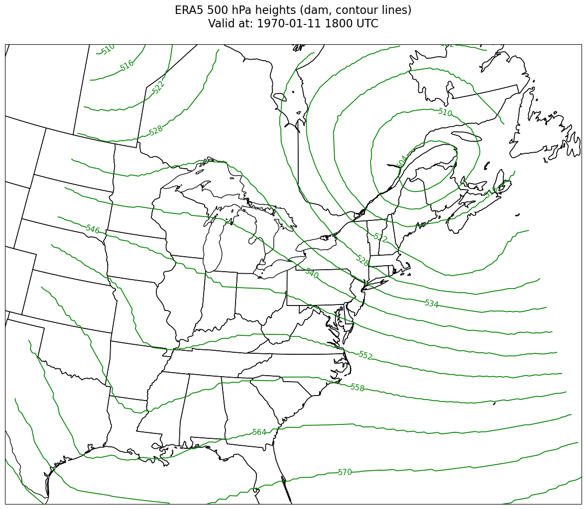
constrainLon = 7 # trial and error!

proj_map = ccrs.LambertConformal(central_longitude=cLon, central_latitude=cLat)
proj_data = ccrs.PlateCarree()
res = '50m'
fig = plt.figure(figsize=(18,12))
ax = plt.subplot(1,1,1,projection=proj_map)
ax.set_extent ([lonW+constrainLon,lonE-constrainLon,latS,latN])
ax.add_feature(cfeature.COASTLINE.with_scale(res))
ax.add_feature(cfeature.STATES.with_scale(res))
#CL = ax.contour(lons,lats,z, levels=Zcintervals ,transform=proj_data,linewidths=1.25, colors='green')
CS = ax.contour(lons,lats,smth, levels=Zcintervals,transform=proj_data,linewidths=1.25, colors='purple')
ax.clabel(CS, inline_spacing=0.2, fontsize=11, fmt='%.0f')
title = plt.title(title_line,fontsize=16)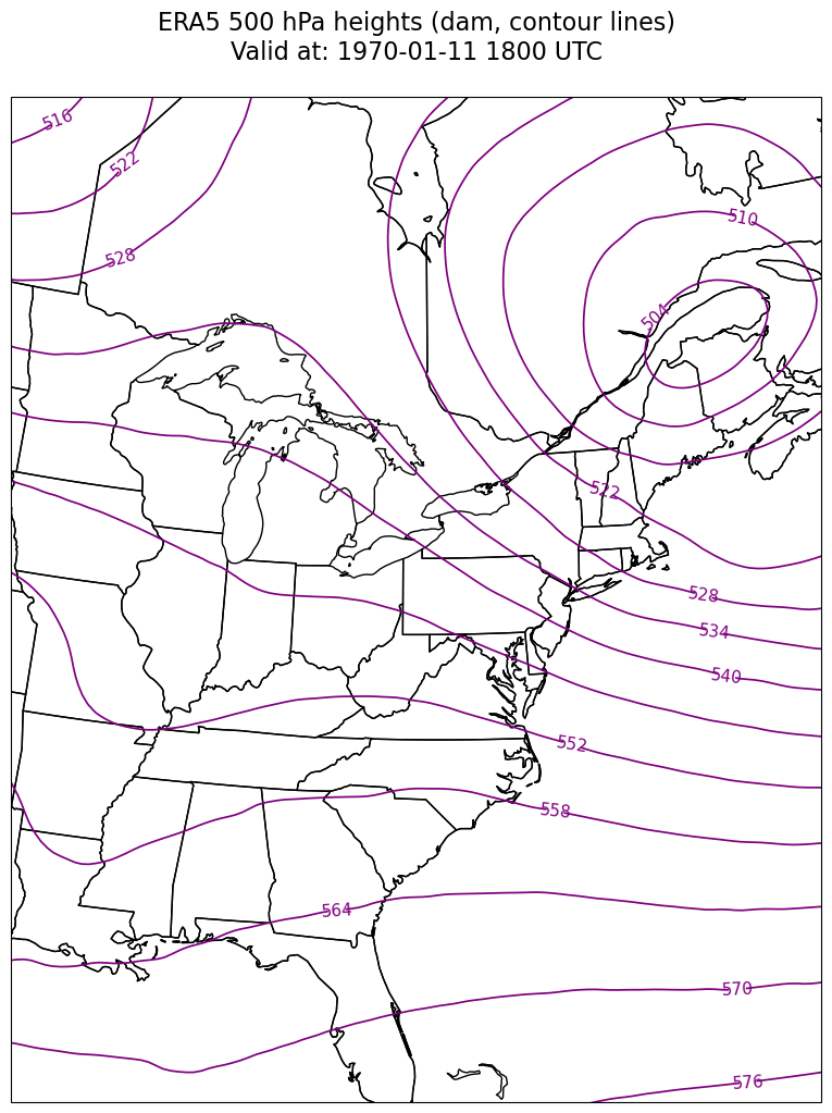
constrainLon = 7 # trial and error!

proj_map = ccrs.LambertConformal(central_longitude=cLon, central_latitude=cLat)
proj_data = ccrs.PlateCarree()
res = '50m'
fig = plt.figure(figsize=(18,12))
ax = plt.subplot(1,1,1,projection=proj_map)
ax.set_extent ([lonW+constrainLon,lonE-constrainLon,latS,latN])
ax.add_feature(cfeature.COASTLINE.with_scale(res))
ax.add_feature(cfeature.STATES.with_scale(res))
CL = ax.contour(lons,lats,z, levels=Zcintervals,transform=proj_data,linewidths=1.25, colors='green')
ax.clabel(CL, inline_spacing=0.2, fontsize=11, fmt='%.0f')
title = plt.title(title_line,fontsize=16)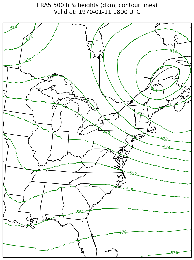
constrainLon = 7 # trial and error!

proj_map = ccrs.LambertConformal(central_longitude=cLon, central_latitude=cLat)
proj_data = ccrs.PlateCarree()
res = '50m'
fig = plt.figure(figsize=(18,12))
ax = plt.subplot(1,1,1,projection=proj_map)
ax.set_extent ([lonW+constrainLon,lonE-constrainLon,latS,latN])
ax.add_feature(cfeature.COASTLINE.with_scale(res))
ax.add_feature(cfeature.STATES.with_scale(res))
CL = ax.contour(lons,lats,z, levels=Zcintervals,transform=proj_data,linewidths=1.25, colors='green')
ax.clabel(CL, inline_spacing=0.2, fontsize=11, fmt='%.0f')
title = plt.title(title_line,fontsize=16)
Things to try:
- Change the date and time
- Change the region
- Use a different map projection for your plot
- Select and overlay different variables
- Very interesting Compare the look of the Destination Earth-sourced dataset versus that from WeatherBench. Do they look the same? Might there be some concerns you have about using one source versus the other?
- Stern, C., Abernathey, R., Hamman, J., Wegener, R., Lepore, C., Harkins, S., & Merose, A. (2022). Pangeo Forge: Crowdsourcing Analysis-Ready, Cloud Optimized Data Production. Frontiers in Climate, 3. 10.3389/fclim.2021.782909