ATM 623: Climate Modeling
Brian E. J. Rose, University at Albany
Lecture 4: Components of the climate system
Tuesday February 10, 2015
About these notes:
This document uses the interactive IPython notebook format (now also called Jupyter). The notes can be accessed in several different ways:
- The interactive notebooks are hosted on
githubat https://github.com/brian-rose/ClimateModeling_courseware - The latest versions can be viewed as static web pages rendered on nbviewer
- A complete snapshot of the notes as of May 2015 (end of spring semester) are available on Brian's website.
Many of these notes make use of the climlab package, available at https://github.com/brian-rose/climlab
1. The climate system and its interactions
Definition of the “climate system”:
From the IPCC AR5 report:
Climate System: “The climate system is the highly complex system consisting of five major components: the atmosphere, the hydrosphere, the cryosphere, the lithosphere and the biosphere, and the interactions between them. The climate system evolves in time under the influence of its own internal dynamics and because of external forcings such as volcanic eruptions, solar variations and anthropogenic forcings such as the changing composition of the atmosphere and land use change.”
Which begs some further definitions:
Atmosphere:
The gaseous envelope surrounding the Earth.
Hydrosphere:
The component of the climate system comprising liquid surface and subterranean water, such as oceans, seas, rivers, lakes, underground water, etc.
Biosphere (terrestrial and marine):
The part of the Earth system comprising all ecosystems and living organisms… including derived dead organic matter, such as litter, soil organic matter and oceanic detritus.
Cryosphere:
All regions on and beneath the surface of the Earth and ocean where water is in solid form, including sea ice, lake ice, river ice, snow cover, glaciers and ice sheets, and frozen ground (which includes permafrost).
Lithosphere:
The upper layer of the solid Earth, both continental and oceanic, which comprises all crustal rocks and the cold, mainly elastic part of the uppermost mantle.
Let’s think about WHY we should want to include all these “spheres” into our models.
Here are two nice figures from the IPCC AR5 WG1 report:
from IPython.display import Image
Image(url='http://www.climatechange2013.org/images/figures/WGI_AR5_Fig1-1.jpg', width=1000)
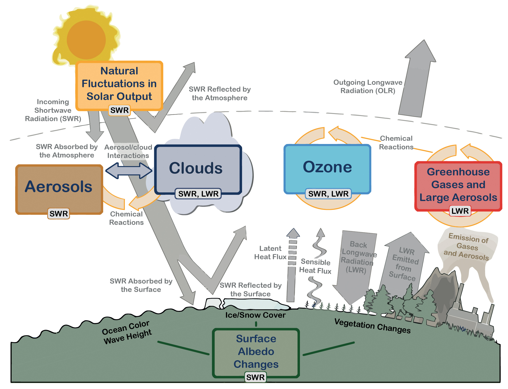
Figure 1.1 | Main drivers of climate change. The radiative balance between incoming solar shortwave radiation (SWR) and outgoing longwave radiation (OLR) is influenced by global climate ‘drivers’. Natural fluctuations in solar output (solar cycles) can cause changes in the energy balance (through fluctuations in the amount of incoming SWR) (Section 2.3). Human activity changes the emissions of gases and aerosols, which are involved in atmospheric chemical reactions, resulting in modified O3 and aerosol amounts (Section 2.2). O3 and aerosol particles absorb, scatter and reflect SWR, changing the energy balance. Some aerosols act as cloud condensation nuclei modifying the properties of cloud droplets and possibly affecting precipitation (Section 7.4). Because cloud interactions with SWR and LWR are large, small changes in the properties of clouds have important implications for the radiative budget (Section 7.4). Anthropogenic changes in GHGs (e.g., CO2, CH4, N2O, O3, CFCs) and large aerosols (>2.5 μm in size) modify the amount of outgoing LWR by absorbing outgoing LWR and re-emitting less energy at a lower temperature (Section 2.2). Surface albedo is changed by changes in vegetation or land surface properties, snow or ice cover and ocean colour (Section 2.3). These changes are driven by natural seasonal and diurnal changes (e.g., snow cover), as well as human influence (e.g., changes in vegetation types) (Forster et al., 2007).
Image(url='http://www.climatechange2013.org/images/figures/WGI_AR5_Fig1-2.jpg', width=1000)

Figure 1.2 | Climate feedbacks and timescales. The climate feedbacks related to increasing CO2 and rising temperature include negative feedbacks (–) such as LWR, lapse rate (see Glossary in Annex III), and air–sea carbon exchange and positive feedbacks (+) such as water vapour and snow/ice albedo feedbacks. Some feedbacks may be positive or negative (±): clouds, ocean circulation changes, air–land CO2 exchange, and emissions of non-GHGs and aerosols from natural systems. In the smaller box, the large difference in timescales for the various feedbacks is highlighted.
The key is that all these processes ultimately affect the planetary energy budget.
Let’s talk about timescales.
Note that the IPCC figure only goes out to centuries – deep ocean circulation – but there are many even longer timescales in the climate system. e.g. growth and decay of ice sheets, geological processes like chemical weathering, continental drift
The choice of which processes to include in a model should therefore be guided by the timescales of interest. For example, the IPCC process is primarily concerned with the century timescale – because it is of special concern to human affairs. So we don’t tend to include ice sheet and geological feedbacks – though coupled ice sheet modeling is becoming more important.
2. Simulation versus Parameterization
Best to discuss this with a specific example: poleward heat transport
We know that the atmosphere moves a lot of energy from warm low latitudes to cold high latitudes – about 5 PW = 10$^{15}$ W actually. This transport of energy mainly occurs in transient weather systems (cyclones and anticyclones), in which warm, moist air tends to move poleward and cold, dry air tends to move equatorward. (we will look at this more careful later in the semester)
Just about every climate model needs to account for this transport and its effects on the energy budgets in any climate model (unless we are dealing ONLY with global averages).
So how can we do it?
Parameterization:
Represent the net effect of many weather systems with an empirical relationship, such as diffusion down mean temperature gradient
Say $T(y)$ is zonally averaged temperature, $y$ is latitude
Transport = $K~dT/dy$
Use observed transport to choose an appropriate value for $K$
- Pro: simple to implement, easy to understand the result
- Con: how might the value of $K$ change with climate change? We have no way of knowing, and have to make assumptions.
Simulation:
Solve the time-dependent equations of motion on a grid of sufficient spatial resolution to represent the growth and decay of synoptic-scale weather systems.
- Pro: model is based on real physical principles (Newton’s laws of motion, conservation of mass and energy). It is therefore more likely to remain valid under changing climate conditions.
- Con: requires lots of computer resources. Must simulate the weather even though we really just want the climate (statistics of weather!)
Essentially a simulation involves representing (at least some aspects of) the underlying rules that govern the process. There is a chain of causality linking input to output.
Parameterization involves making assumptions about the statistical properties of the process – so we can calculate some relevant statistical properties of the output given the input, without needing to explicitly model the actual events.
3. Introducing the GCM
GCM:
Depending on who you ask, it is either:
- General Circulation Model (the original)
- Global Climate Model (more common these days)
The reading from the Climate Modelling Primer spells out the history of the development of GCMs:
- started out as atmospheric models and separate ocean models
- gradually more and more processes are being coupled together.
- This leads to incredibly complex pieces of software, running on some of the world’s largest computer clusters.
Image(url='http://www.climatechange2013.org/images/figures/WGI_AR5_Fig1-13.jpg', width=1000)

Figure 1.13 | The development of climate models over the last 35 years showing how the different components were coupled into comprehensive climate models over time. In each aspect (e.g., the atmosphere, which comprises a wide range of atmospheric processes) the complexity and range of processes has increased over time (illustrated by growing cylinders). Note that during the same time the horizontal and vertical resolution has increased considerably e.g., for spectral models from T21L9 (roughly 500 km horizontal resolu- tion and 9 vertical levels) in the 1970s to T95L95 (roughly 100 km horizontal resolution and 95 vertical levels) at present, and that now ensembles with at least three independent experiments can be considered as standard.
Image(url='http://www.climatechange2013.org/images/figures/WGI_AR5_Fig1-14.jpg', width=1000)
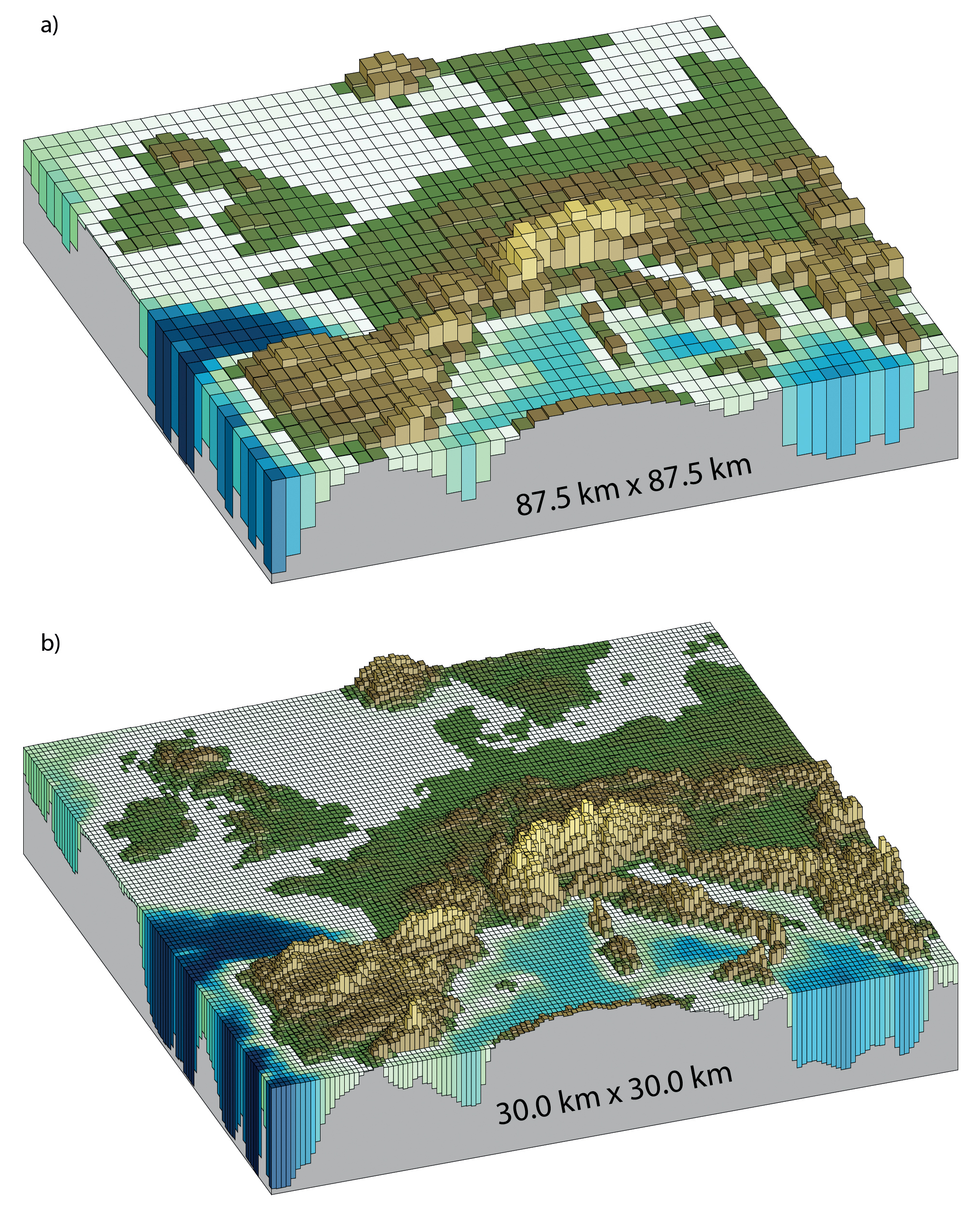
Figure 1.14 | Horizontal resolutions considered in today’s higher resolution models and in the very high resolution models now being tested: (a) Illustration of the European topography at a resolution of 87.5 × 87.5 km; (b) same as (a) but for a resolution of 30.0 × 30.0 km.
One goal of all this complexity is to do more simulation and less parameterization in order to get a more accurate prediction of climate change.
In terms of our simple view of planetary energy budget, we are trying to represent the net climate feedback $\lambda$ correctly, and so get the correct climate sensitivity.
Ideally this means basing the model on laws of physics and chemistry.
However it doesn’t always work this way. In many cases we know that a feedback operates in nature, but we can’t represent it in terms of first principles.
Land surface processes are a good example.
Exchanges of energy, water and carbon between the land and atmosphere are biologically mediated. We must (to a certain extent) rely on empirical relationships. A bit like economic modeling.
We also must deal with interaction across spatial scales.
E.g. cumulus convection and vertical transport of heat and water vapor
4. The Community Earth System Model (CESM)
What is it?
- CESM is one of a handful of complex coupled GCMs that are used as part of the IPCC process.
- Developed and maintained at NCAR (Boulder CO) by a group of climate scientists and software engineers.
- “Community” refers to the fact that the code is open-source, with new pieces contributed by a wide variety of users.
I use CESM in my own research. We are going to be using CESM in this course. Everyone should visit the website and learn about it.
Key components of CESM: (or any equivalent modern GCM)
- Atmospheric model, AGCM
- Ocean model, OGCM
- Land surface model
- Sea ice model
The software is somewhat modular, so different submodels can be combined together depending on the nature of the scientific problem at hand and the available computer power.
E.g. we can run the model in “atmosphere-only” mode. Surface conditions over land and ocean will be prescribed from observations. It is difficult to learn much about climate change this way.
Why?
Because the surface temperature can’t change in response to energy imbalance!
i.e. it’s not a climate model, according to our working definition.
Let’s say we want to use our model to estimate equilibrium climate sensitivity. Recall $\Delta T_{2\times CO_2}$ is the warming we get from doubling atmospheric CO2, once the planetary energy budget has adjusted back to equilibrium.
In this class we will mostly work with the so-called slab ocean model.
You got introduced to this model in the homework exercise.
The key is that we allow the sea surface temperature to change, but we fix (prescribe) the net effect of ocean currents on the transport of energy.
Why do this?
Because it takes thousands of years for the full ocean model to come into equilibrium!
Why should we believe the results of the slab ocean model?
We shouldn’t!
But experience with coupled models (meaning interactive ocean circulation) has shown that the circulation does not change radically under $2\times CO_2$.
So the slab ocean model gives us a decent first guess at climate sensitivity. And it makes it possible to do a lot of experimentation that we wouldn’t be able to do otherwise.
5. Our numerical experiments with CESM
Atmosphere
- Horizontal resolution about 2º lat/lon
- AGCM solves the fundamental equations:
- Conservation of momentum, mass, energy, water, equation of state
- At 2º we resolve the synoptic-scale dynamics
- storm tracks and cyclones.
- We do NOT resolve the mesoscale and smaller
- thunderstorms, individual convective events, clouds
- These all must be parameterized.
- Model also solves equations of radiative transfer. This takes account of
- composition of the atmosphere and the absorption properties of different gases
- radiative effects of clouds.
Sea ice
- Resolution of 1º.
- Thermodynamics (conservation of energy, water and salt)
- determines freezing and melting
- Dynamics (momentum equations)
- determine ice motion and deformation.
- Complex! Sea ice is sort of a mixture of a fluid and a solid.
Land surface model
- Same resolution as atmosphere.
- Determines surface fluxes of heat, water, momentum (friction) based on prescribed vegetation types.
- Don’t actually know much about how it works!
- Great topic for someone to dig in to for their term project.
Ocean
- Same grid as sea ice, 1º.
- Sea surface temperature evolves based on:
- heat exchange with atmosphere
- prescribed “q-flux”.
Experimental setup
Model is given realistic atmospheric composition, realistic solar radiation, etc.
We perform a control run to get a baseline simulation, and take averages of several years (because the model has internal variability – every year is a little bit different)
We then change something, e.g. $2\times CO_2$!
And allow the model to adjust to a new equilibrium, just as we did with the toy energy balance model.
Once it has gotten close to its new equilibrium, we run it for several more years again to get the new climatology.
Then we can look at the differences in the climatologies before and after the perturbation.
5. What can we resolve with a 2º atmosphere?
The following animation shows contours of sea level pressure in the control simulation. It is based on 6-hourly output from the numerical model.
The atmosphere is simulated with a 2º finite volume dynamical core.
from IPython.display import YouTubeVideo
YouTubeVideo('As85L34fKYQ')
Discussion point:
How well does this represent the true general circulation of the atmosphere?
Citation information
The figures above are reproduced from Chapter 1 of the IPCC AR5 Working Group 1 report. The report and images can be found online at http://www.climatechange2013.org/report/full-report/
The full citation is:
Cubasch, U., D. Wuebbles, D. Chen, M.C. Facchini, D. Frame, N. Mahowald and J.-G. Winther, 2013: Introduction. In: Climate Change 2013: The Physical Science Basis. Contribution of Working Group I to the Fifth Assessment Report of the Intergovernmental Panel on Climate Change [Stocker, T.F., D. Qin, G.-K. Plattner, M. Tignor, S.K. Allen, J. Boschung, A. Nauels, Y. Xia, V. Bex and P.M. Midgley (eds.)]. Cambridge University Press, Cambridge, United Kingdom and New York, NY, USA, pp. 119–158, doi:10.1017/CBO9781107415324.007.
%install_ext http://raw.github.com/jrjohansson/version_information/master/version_information.py
%load_ext version_information
%version_information numpy, climlab
Credits
The author of this notebook is Brian E. J. Rose, University at Albany.
It was developed in support of ATM 623: Climate Modeling, a graduate-level course in the Department of Atmospheric and Envionmental Sciences, offered in Spring 2015.