Introduction to Cartopy

Overview¶

Basic concepts: map projections and GeoAxes
Explore some of Cartopy’s map projections
Create regional maps

This tutorial will lead you through some basics of creating maps with specified projections with Cartopy, and adding geographic features like coastlines and borders.

Later tutorials will focus on how to plot data on map projections.

Prerequisites¶

Concepts	Importance	Notes
Matplotlib	Necessary

Time to learn: 30 minutes

Imports¶

import matplotlib.pyplot as plt
import pandas as pd
from cartopy import crs as ccrs, feature as cfeature

#  Suppress warnings issued by Cartopy when downloading data files
import warnings
warnings.filterwarnings('ignore')

Motivation: consider the following `DataFrame`:¶

locations = pd.read_csv('/spare11/atm350/common/data/locs.csv')

Examine the first few lines of the DataFrame

locations

Loading...

# Write your code below. 
lats = locations['lat']
lons = locations['lon']

Click to reveal only AFTER you have tried your own code!

lats = locations['lat']
lons = locations['lon']

Examine one of the Series.

lons

0     -77.237260
1     -74.801390
2     -78.135660
3     -73.945270
4     -75.668520
         ...    
122   -73.858829
123   -75.158597
124   -73.423071
125   -76.842610
126   -77.847760
Name: lon, Length: 127, dtype: float64

Use Matplotlib’s ax.scatter function to plot these points on a figure.

fig = plt.figure(figsize=(11,8.5))
ax = fig.add_subplot(1,1,1)
ax.scatter(lons, lats)
ax.set_title("What does this make you think of??")
ax.set_xlabel('Longitudes')
ax.set_ylabel('Latitudes');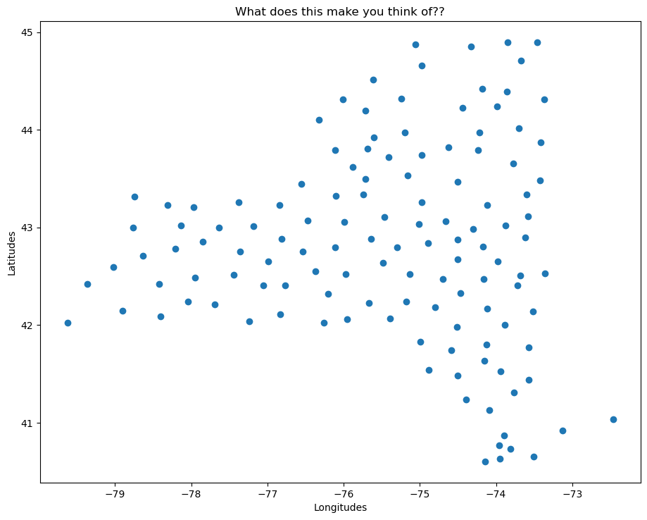

We can get a sense that this looks like a map! However, all we have here are x- and y- coordinate pairs, which just so happen to have values that resemble longitudes and latitudes, in degrees. Matplotlib, by itself, does not provide mapmaking (i.e., cartographic) functionality. We will use a separate package, Cartopy, which extends Matplotlib’s two-dimensional `Axes` into a cartographic context ... i.e., geo-referenced `GeoAxes`.¶

Recall that in Matplotlib, what we might tradtionally term a figure consists of two key components: a figure and an associated subplot axes instance.

By virtue of importing Cartopy, we can now convert the axes into a GeoAxes by specifying a map projection that we have imported from Cartopy’s Coordinate Reference System class (ccrs). This will effectively georeference the subplot.

Create a map with a specified projection¶

Here we’ll create a GeoAxes that uses the PlateCarree projection (basically a global lat-lon map projection, which translates from French to “flat square” in English, where each point is equally spaced in terms of degrees).

fig = plt.figure(figsize=(11, 8.5))
ax = plt.subplot(1, 1, 1, projection=ccrs.PlateCarree(central_longitude=-75))
ax.set_title("A Geo-referenced subplot, Plate Carree projection");

Although the figure seems empty, it has in fact been georeferenced, using one of Cartopy’s map projections that is provided by Cartopy’s crs (coordinate reference system) class. We can now add in cartographic features, in the form of shapefiles, to our subplot. One of them is coastlines, which is a callable GeoAxes method that can be plotted directly on our subplot.

ax.coastlines()

<cartopy.mpl.feature_artist.FeatureArtist at 0x152d7d0a3b60>

fig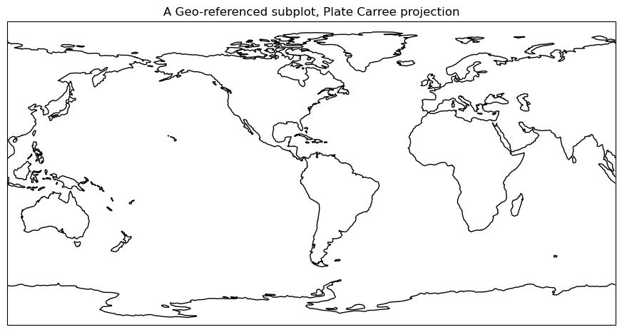

Add cartographic features to the map¶

Cartopy provides other cartographic features via its features class, which we’ve imported as cfeature. These are also shapefiles, downloaded on initial request from https://www.naturalearthdata.com/. Once downloaded, they typically “live” in your ~/.local/share/cartopy directory (note the ~ represents your home directory).

We add them to our subplot via the add_feature method. We can define attributes for them in a manner similar to Matplotlib’s plot method. A list of the various Natural Earth shapefiles appears in https://scitools.org.uk/cartopy/docs/latest/matplotlib/feature_interface.html .

ax.add_feature(cfeature.BORDERS, linewidth=0.5, edgecolor='black')
ax.add_feature(cfeature.STATES, linewidth=0.3, edgecolor='brown')

<cartopy.mpl.feature_artist.FeatureArtist at 0x152d74bca850>

Once again, referencing the Figure object will re-render the figure in the notebook, now including the two features.

fig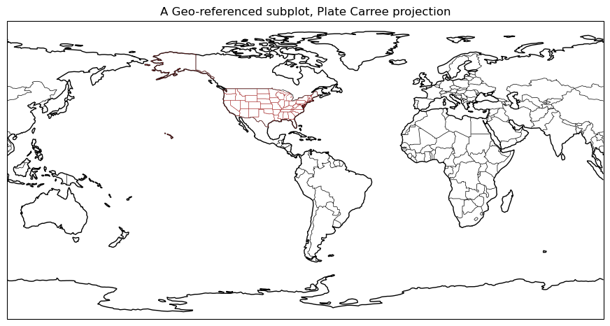

Explore some of Cartopy’s map projections¶

Mollweide Projection (often used with global satellite mosaics)¶

This time, we’ll define an object to store our projection definition. Any time we wish to use this particular projection later in the notebook, we can use the object name rather than repeating the same call to ccrs.

fig = plt.figure(figsize=(11, 8.5))
projMoll = ccrs.Mollweide(central_longitude=-137.8)
ax = plt.subplot(1, 1, 1, projection=projMoll)
ax.set_title("Mollweide Projection")

Add in the cartographic shapefiles¶

ax.coastlines()
ax.add_feature(cfeature.BORDERS, linewidth=0.5, edgecolor='blue')
fig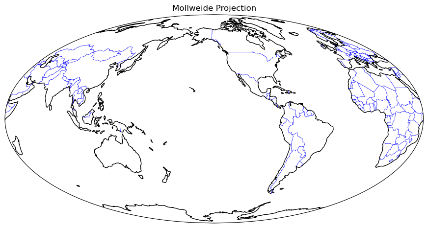

Add a fancy background image to the map.¶

ax.stock_img()
fig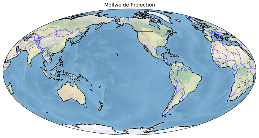

Lambert Azimuthal Equal Area Projection¶

fig = plt.figure(figsize=(11, 8.5))
projLae = ccrs.LambertAzimuthalEqualArea(central_longitude=0.0, central_latitude=0.0)
ax = plt.subplot(1, 1, 1, projection=projLae)
ax.set_title("Lambert Azimuthal Equal Area Projection")
ax.coastlines()
ax.add_feature(cfeature.BORDERS, linewidth=0.5, edgecolor='blue');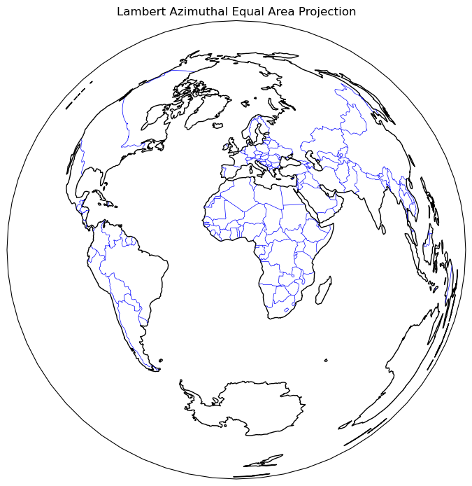

Create regional maps¶

Cartopy’s `set_extent` method¶

Now, let’s go back to PlateCarree, but let’s use Cartopy’s set_extent method to restrict the map coverage to a North American view. Let’s also choose a lower resolution for coastlines, just to illustrate how one can specify that. Plot lat/lon lines as well.

Reference for Natural Earth’s three resolutions (10m, 50m, 110m; higher is coarser): https://www.naturalearthdata.com/downloads/

projPC = ccrs.PlateCarree()
lonW = -140
lonE = -40
latS = 15
latN = 65
cLat = (latN + latS) / 2
cLon = (lonW + lonE) / 2
res = '110m'

fig = plt.figure(figsize=(11, 8.5))
ax = plt.subplot(1, 1, 1, projection=projPC)
ax.set_title('Plate Carree')
gl = ax.gridlines(
    draw_labels=True, linewidth=2, color='gray', alpha=0.5, linestyle='--'
)
ax.set_extent([lonW, lonE, latS, latN], crs=projPC)
ax.coastlines(resolution=res, color='black')
ax.add_feature(cfeature.STATES, linewidth=0.3, edgecolor='brown')
ax.add_feature(cfeature.BORDERS, linewidth=0.5, edgecolor='blue');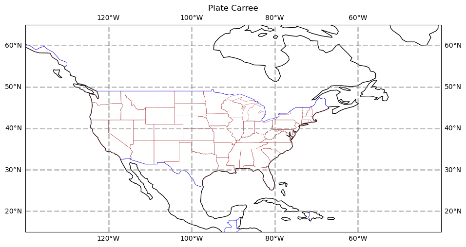

The PlateCarree projection exaggerates the spatial extent of regions closer to the poles. Let’s try a couple different projections.

projStr = ccrs.Stereographic(central_longitude=cLon, central_latitude=cLat)
fig = plt.figure(figsize=(11, 8.5))
ax = plt.subplot(1, 1, 1, projection=projStr)
ax.set_title('Stereographic')
gl = ax.gridlines(
    draw_labels=True, linewidth=2, color='gray', alpha=0.5, linestyle='--'
)
ax.set_extent([lonW, lonE, latS, latN], crs=projPC)
ax.coastlines(resolution=res, color='black')
ax.add_feature(cfeature.STATES, linewidth=0.3, edgecolor='brown')
ax.add_feature(cfeature.BORDERS, linewidth=0.5, edgecolor='blue');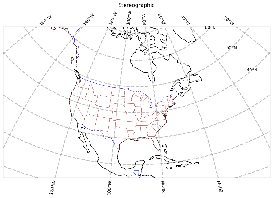

projLcc = ccrs.LambertConformal(central_longitude=cLon, central_latitude=cLat)
fig = plt.figure(figsize=(11, 8.5))
ax = plt.subplot(1, 1, 1, projection=projLcc)
ax.set_title('Lambert Conformal')
gl = ax.gridlines(
    draw_labels=True, linewidth=2, color='gray', alpha=0.5, linestyle='--'
)
ax.set_extent([lonW, lonE, latS, latN], crs=projPC)
ax.coastlines(resolution='110m', color='black')
ax.add_feature(cfeature.STATES, linewidth=0.3, edgecolor='brown')
# End last line with a semicolon to suppress text output to the screen
ax.add_feature(cfeature.BORDERS, linewidth=0.5, edgecolor='blue');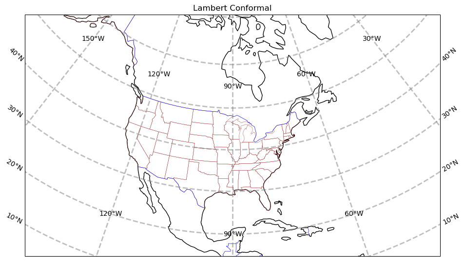

Create a regional map centered over New York State¶

Set the domain for defining the plot region. We will use this in the set_extent line below. Since these coordinates are expressed in degrees, they correspond to the PlateCarree projection.

latN = 45.2
latS = 40.2
lonW = -80.0
lonE = -71.5
cLat = (latN + latS) / 2
cLon = (lonW + lonE) / 2
projLccNY = ccrs.LambertConformal(central_longitude=cLon, central_latitude=cLat)

Add some pre-defined Features¶

Some pre-defined Features exist as cartopy.feature constants. The resolution of these pre-defined Features will depend on the areal extent of your map, which you specify via set_extent.

fig = plt.figure(figsize=(15, 10))
ax = plt.subplot(1, 1, 1, projection=projLccNY)
ax.set_extent([lonW, lonE, latS, latN], crs=projPC)
ax.set_facecolor(cfeature.COLORS['water'])
# Ocean feature is commented out ... see note below
# ax.add_feature(cfeature.OCEAN)
ax.add_feature(cfeature.LAND)
ax.add_feature(cfeature.COASTLINE)
ax.add_feature(cfeature.BORDERS, linestyle='--')
ax.add_feature(cfeature.LAKES, alpha=0.5)
ax.add_feature(cfeature.STATES)
ax.add_feature(cfeature.RIVERS)
ax.set_title('New York and Vicinity');

Use lower resolution shapefiles from Natural Earth¶

Let’s create a new map, but this time use lower-resolution shapefiles from Natural Earth, and also eliminate plotting the country borders.

Notice this is a bit more involved. First we create objects for our lower-resolution shapefiles via the NaturalEarthFeature method from Cartopy’s feature class, and then we add them to the map with add_feature.

fig = plt.figure(figsize=(15, 10))
ax = plt.subplot(1, 1, 1, projection=projLccNY)
ax.set_extent((lonW, lonE, latS, latN), crs=projPC)

# The features with names such as cfeature.LAND, cfeature.OCEAN, are higher-resolution (10m)
# shapefiles from the Naturalearth repository.  Lower resolution shapefiles (50m, 110m) can be
# used by using the cfeature.NaturalEarthFeature method as illustrated below.

resolution = '110m'

land_mask = cfeature.NaturalEarthFeature(
    'physical',
    'land',
    scale=resolution,
    edgecolor='face',
    facecolor=cfeature.COLORS['land'],
)
sea_mask = cfeature.NaturalEarthFeature(
    'physical',
    'ocean',
    scale=resolution,
    edgecolor='face',
    facecolor=cfeature.COLORS['water'],
)
lake_mask = cfeature.NaturalEarthFeature(
    'physical',
    'lakes',
    scale=resolution,
    edgecolor='face',
    facecolor=cfeature.COLORS['water'],
)
state_borders = cfeature.NaturalEarthFeature(
    category='cultural',
    name='admin_1_states_provinces_lakes',
    scale=resolution,
    facecolor='none',
)

ax.add_feature(land_mask)
ax.add_feature(sea_mask)
ax.add_feature(lake_mask)
ax.add_feature(state_borders, linestyle='solid', edgecolor='black')
ax.set_title('New York and Vicinity; lower resolution');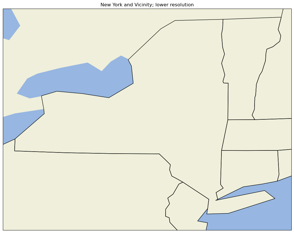

A figure with two different regional maps¶

Finally, let’s create a figure with two subplots. On one, we’ll repeat our hi-res NYS map; on the second, we’ll plot over a different part of the world.

# Create the figure object
fig = plt.figure(
    figsize=(30, 24)
)  # Notice we need a bigger "canvas" so these two maps will be of a decent size

# First subplot
ax = plt.subplot(2, 1, 1, projection=projLccNY)
ax.set_extent([lonW, lonE, latS, latN], crs=projPC)
ax.set_facecolor(cfeature.COLORS['water'])
ax.add_feature(cfeature.LAND)
ax.add_feature(cfeature.COASTLINE)
ax.add_feature(cfeature.BORDERS, linestyle='--')
ax.add_feature(cfeature.LAKES, alpha=0.5)
ax.add_feature(cfeature.STATES)
ax.set_title('New York and Vicinity')

# Set the domain for defining the second plot region.
latN = 70
latS = 30.2
lonW = -10
lonE = 50
cLat = (latN + latS) / 2
cLon = (lonW + lonE) / 2

projLccEur = ccrs.LambertConformal(central_longitude=cLon, central_latitude=cLat)

# Second subplot
ax2 = plt.subplot(2, 1, 2, projection=projLccEur)
ax2.set_extent([lonW, lonE, latS, latN], crs=projPC)
ax2.set_facecolor(cfeature.COLORS['water'])
ax2.add_feature(cfeature.LAND)
ax2.add_feature(cfeature.COASTLINE)
ax2.add_feature(cfeature.BORDERS, linestyle='--')
ax2.add_feature(cfeature.LAKES, alpha=0.5)
ax2.add_feature(cfeature.STATES)
ax2.set_title('Europe');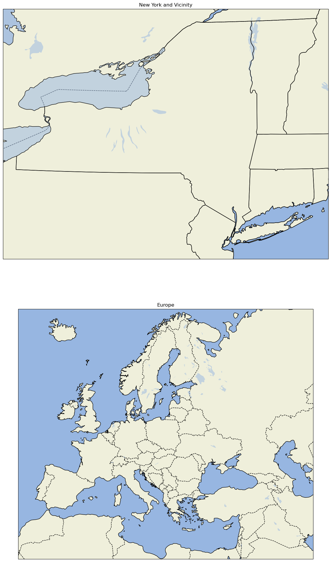

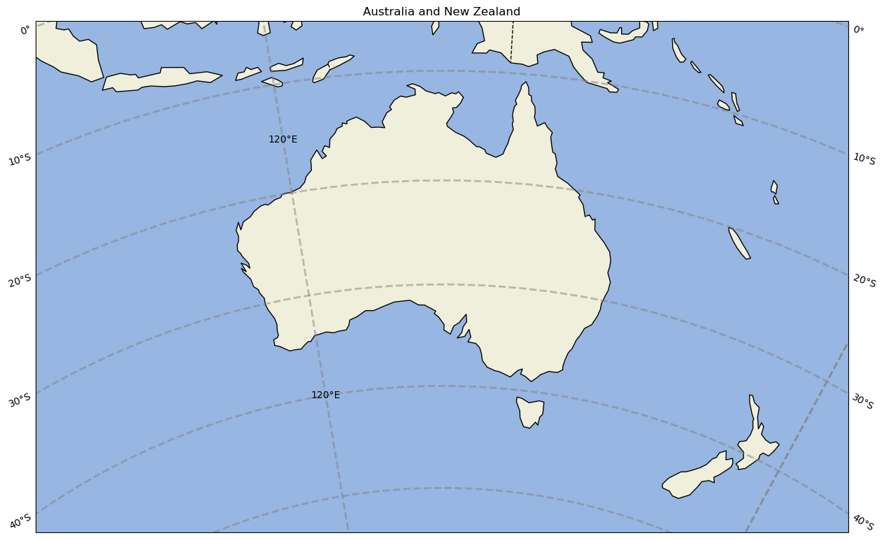
Create a single-panel figure centered over Australia and New Zealand¶

# Create the figure object
fig = plt.figure(
    figsize=(15, 12)
)  

# Set the domain for defining the plot region.
latN = -5
latS = -50
lonW = 100
lonE = 170
cLat = (latN + latS) / 2
cLon = (lonW + lonE) / 2


# Use non-default values for standard_parallels and cutoff latitudes for southern hemisphere regions
projANZ = ccrs.LambertConformal(central_longitude=cLon, central_latitude=cLat, standard_parallels=(-33,-45), cutoff=30)

ax = plt.subplot(1, 1, 1, projection=projANZ)

ax.set_extent([lonW, lonE, latS, latN], crs=ccrs.PlateCarree())
ax.set_facecolor(cfeature.COLORS['water'])
ax.add_feature(cfeature.LAND)
ax.add_feature(cfeature.COASTLINE)
ax.add_feature(cfeature.BORDERS, linestyle='--')
ax.add_feature(cfeature.LAKES, alpha=0.5)
ax.add_feature(cfeature.STATES)
ax.gridlines(draw_labels=True, linewidth=2, color='gray', alpha=0.5, linestyle='--')
ax.set_title('Australia and New Zealand');

# Write your code below

Summary¶

Cartopy allows for georeferencing Matplotlib axes objects.
Cartopy’s crs class supports a variety of map projections.
Cartopy’s feature class allows for a variety of cartographic features to be overlaid on the figure.

What’s Next?¶

In the next notebook, we will plot data from the NYS Mesonet. Additionally, we will delve further into how one can transform data that is defined in one coordinate reference system (crs) so it displays properly on a map that uses a different crs.

Overview¶

Prerequisites¶

Imports¶

Motivation: consider the following DataFrame:¶

Create a map with a specified projection¶

Add cartographic features to the map¶

Explore some of Cartopy’s map projections¶

Mollweide Projection (often used with global satellite mosaics)¶

Add in the cartographic shapefiles¶

Add a fancy background image to the map.¶

Lambert Azimuthal Equal Area Projection¶

Create regional maps¶

Cartopy’s set_extent method¶

Create a regional map centered over New York State¶

Add some pre-defined Features¶

Use lower resolution shapefiles from Natural Earth¶

A figure with two different regional maps¶

Create a single-panel figure centered over Australia and New Zealand¶

Summary¶

What’s Next?¶

Motivation: consider the following `DataFrame`:¶

Cartopy’s `set_extent` method¶