04_GriddedDiagnostics_Frontogenesis_ERA5
Overview
Select a date and access the ERA5 dataset
Subset the desired variables along their dimensions
Calculate and visualize diagnostic quantities.
Imports
import xarray as xr
import pandas as pd
import numpy as np
from datetime import datetime as dt
from metpy.units import units
import metpy.calc as mpcalc
import cartopy.crs as ccrs
import cartopy.feature as cfeature
import matplotlib.pyplot as plt
Specify a starting and ending date/time, regional extent, vertical levels, and access/subset the ERA5
# 1. Set the bounds of your map.
# Set the four values in the code cell below. Test the values.
latN = 48
latS = 32
lonW = -85
lonE = -60

if ( latN > latS ) and ( lonE > lonW):
    cLat = (latN + latS)/2
    cLon = (lonW + lonE)/2
else:
    e = ("Northern (eastern) latitude (longitude) must be greater than southern (western). Go back and re-adjust!")
    raise ValueError(f"Error in lat/lon specification: {e}")

# Recall that in ERA5, longitudes run between 0 and 360, not -180 and 180
if (lonW < 0 ):
    lonW = lonW + 360
if (lonE < 0 ):
    lonE = lonE + 360

# 2. Select the map projection for your figure.
proj_map = ccrs.LambertConformal(central_latitude=cLat, central_longitude=cLon)

# 3. Select the projection on which the dataset is based
proj_data = ccrs.PlateCarree()

# 4. Select the resolution of the Cartopy cartographic features, and, if desired, MetPy's county shapefiles.

# Uncomment / comment as desired
#res = '10m' # Most detailed, best for small regions (e.g. NYS)
res = '50m' # Medium detail, best for medium-sized regions (e.g. CONUS)
#res = '110m' # Least detailed, best for large/global maps

#res_county = '5m' # Higher-res MetPy US County shapefiles
res_county = '20m' # Lower-res MetPy US County shapefiles

# Apply the latitude/longitude ranges and extend the data region if desired

expand_lon = 1
expand_lat = 1
latRange = np.arange(latS - expand_lat,latN + expand_lat,.25) # expand the data range a bit beyond the plot range
lonRange = np.arange((lonW - expand_lon),(lonE + expand_lon),.25) # Need to match longitude values to those of the coordinate variable

# Specify desired pressure levels: in this case, a list of one or more
plevel_list = [700,850]

startYear = 2026
startMonth = 2
startDay = 23
startHour = 0
startMinute = 0
startDateTime = dt(startYear,startMonth,startDay, startHour, startMinute)

endYear = 2026
endMonth = 2
endDay = 23
endHour = 12
endMinute = 0
endDateTime = dt(endYear,endMonth,endDay, endHour, endMinute)

delta_time = endDateTime - startDateTime
time_range_max = 7*86400

if (delta_time.total_seconds() > time_range_max):
    raise RuntimeError("Your time range must not exceed 7 days. Go back and try again.")

# Create a list of date and times based on what we specified for the initial and final times,
#  using Pandas’ date_range function
dateRange = pd.date_range(startDateTime, endDateTime,freq="6h")
Print out the lat/lon, pressure, and date/time arrays
print ("Summary of subsetted dimensions: \n\n")
print (f'Longitude Range: {lonRange} \n')
print (f'Latitude Range: {latRange} \n')
print (f'Pressure levels: {plevel_list} \n')
print(f'Date Range: {dateRange}')
Summary of subsetted dimensions:
Longitude Range: [274. 274.25 274.5 274.75 275. 275.25 275.5 275.75 276. 276.25
276.5 276.75 277. 277.25 277.5 277.75 278. 278.25 278.5 278.75
279. 279.25 279.5 279.75 280. 280.25 280.5 280.75 281. 281.25
281.5 281.75 282. 282.25 282.5 282.75 283. 283.25 283.5 283.75
284. 284.25 284.5 284.75 285. 285.25 285.5 285.75 286. 286.25
286.5 286.75 287. 287.25 287.5 287.75 288. 288.25 288.5 288.75
289. 289.25 289.5 289.75 290. 290.25 290.5 290.75 291. 291.25
291.5 291.75 292. 292.25 292.5 292.75 293. 293.25 293.5 293.75
294. 294.25 294.5 294.75 295. 295.25 295.5 295.75 296. 296.25
296.5 296.75 297. 297.25 297.5 297.75 298. 298.25 298.5 298.75
299. 299.25 299.5 299.75 300. 300.25 300.5 300.75]
Latitude Range: [31. 31.25 31.5 31.75 32. 32.25 32.5 32.75 33. 33.25 33.5 33.75
34. 34.25 34.5 34.75 35. 35.25 35.5 35.75 36. 36.25 36.5 36.75
37. 37.25 37.5 37.75 38. 38.25 38.5 38.75 39. 39.25 39.5 39.75
40. 40.25 40.5 40.75 41. 41.25 41.5 41.75 42. 42.25 42.5 42.75
43. 43.25 43.5 43.75 44. 44.25 44.5 44.75 45. 45.25 45.5 45.75
46. 46.25 46.5 46.75 47. 47.25 47.5 47.75 48. 48.25 48.5 48.75]
Pressure levels: [700, 850]
Date Range: DatetimeIndex(['2026-02-23 00:00:00', '2026-02-23 06:00:00',
'2026-02-23 12:00:00'],
dtype='datetime64[ns]', freq='6h')
Access either the cloud-served or local ERA5 repository. Then subset it according to your choices above.
endDate = dt(2023,1,10)
if (endDateTime <= endDate): # Use WeatherBench archive

    cloud_source = True
    ds = xr.open_dataset(
     'gs://weatherbench2/datasets/era5/1959-2023_01_10-wb13-6h-1440x721.zarr',
     chunks={'time': 48},
     consolidated=True,
     engine='zarr'
    )

    # Attach units to the pressure coordinate
    ds.coords['level'].attrs['units'] = 'hPa'

    # Rename the variable names in this dataset so they use their corresponding short_name attributes
    # Construct a dictionary whose keys are the original variable names, and whose values are their
    # short names

    rename_data_vars = {}
    seen_short_names = set()

    for var_name in ds.data_vars:
        short = ds[var_name].attrs.get("short_name")
        # Only rename if:
        # 1. short_name exists
        # 2. We haven't already used it
        if short and short not in seen_short_names:
            rename_data_vars[var_name] = short
            seen_short_names.add(short)
    # Apply renaming
    ds = ds.rename(rename_data_vars)

else: # Use local archive
    import glob, os
    cloud_source = False
    input_directory = '/free/ktyle/era5'
    files = glob.glob(os.path.join(input_directory,'*_era5.nc'))
    ds = xr.open_mfdataset(files,coords='minimal',compat='override')
    # Rename two of the coordinate variables so they match what is in the WeatherBench archive
    ds = ds.rename({'valid_time': 'time', 'pressure_level': 'level'})

# Perform the initial subset
ds = ds.sel(time = dateRange, longitude = lonRange, latitude = latRange, level = plevel_list)Examine the subsetted Dataset
dsNow create DataArray objects for the data variables we are interested in. Since we are interested in computing dewpoint, as well as displaying wind barbs, what variables might we require?
# write your code here
T = ds['t']
U = ds['u']
V = ds['v']
In preparation for calculating diagnostics, let’s first select just a single isobaric surface from the four that we previously listed. Subset the data variables based on that level.
p_level = 700
Tp = T.sel(level=p_level).compute()
Up = U.sel(level=p_level).compute()
Vp = V.sel(level=p_level).compute()Calculate potential temperature
Thetap = mpcalc.potential_temperature(Tp.level, Tp)
ThetapCalculate frontogenesis
Frnt = mpcalc.frontogenesis(Thetap, Up, Vp)
FrntLet’s get a quick visualization, using Xarray’s built-in interface to Matplotlib.
Frnt.isel(time=0).plot(figsize=(15,10),cmap='coolwarm')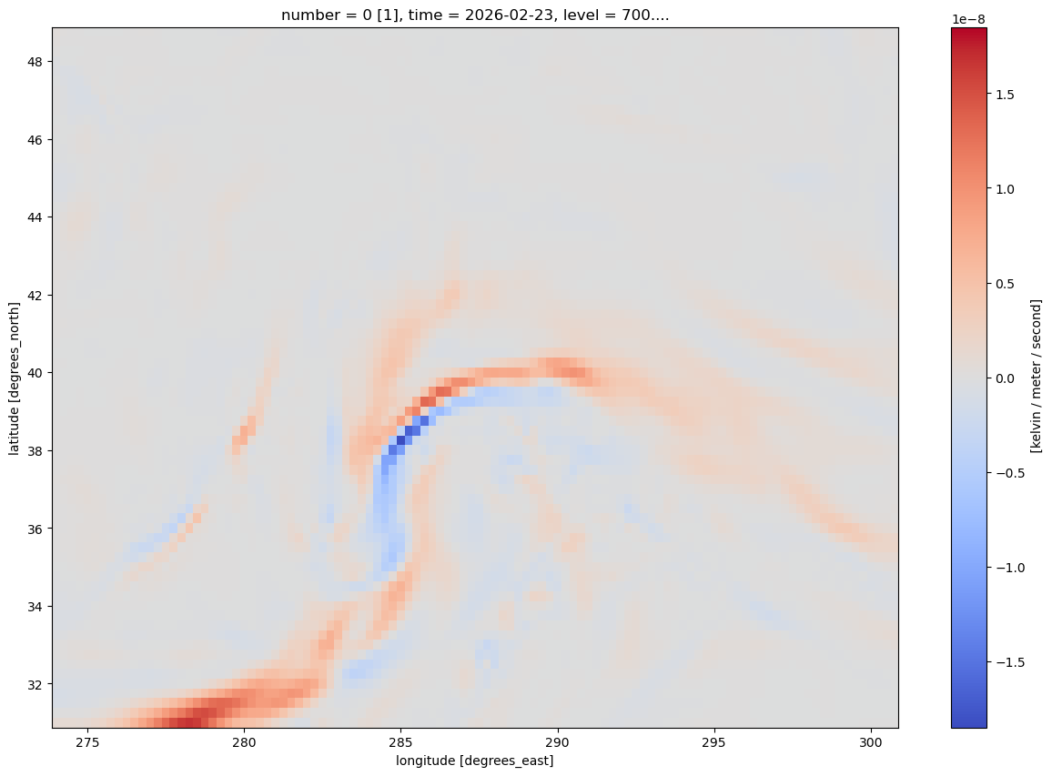
Now, let’s prepare to make a nice-looking map of frontogenesis.
The units are in degrees K (or C) per meter per second. Traditionally, we plot frontogenesis on more of a meso- or synoptic scale … K or degrees C per 100 km per 3 hours. Let’s simply multiply by the conversion factor.
# A conversion factor to get frontogensis units of K per 100 km per 3 h
convert_to_per_100km_3h = 1000*100*3600*3
FrntCnv = Frnt * convert_to_per_100km_3h
Check the range and scale of values.
FrntCnv.min().values, FrntCnv.max().values(array(-21.2142768), array(34.71061552))A scale of 1 (i.e., 1x10^0, AKA 1e0) looks appropriate.
Apply a Gaussian smoother
sigma = 7.0 # this depends on how noisy your data is, adjust as necessary
FrntSmth = mpcalc.smooth_gaussian(FrntCnv, sigma)
Find the min/max of the scaled and smoothed values. Use these to inform the setting of the contour fill intervals.
scale = 1e0
minFrnt= (FrntSmth*scale).min().values
maxFrnt = (FrntSmth*scale).max().values
print (minFrnt, maxFrnt)
-11.559388114841418 18.62756235181785
# Avoid the zero contour line, or filled contours that straddle 0
frntInc = 3
negFrntContours = np.arange (-21, 0, frntInc)
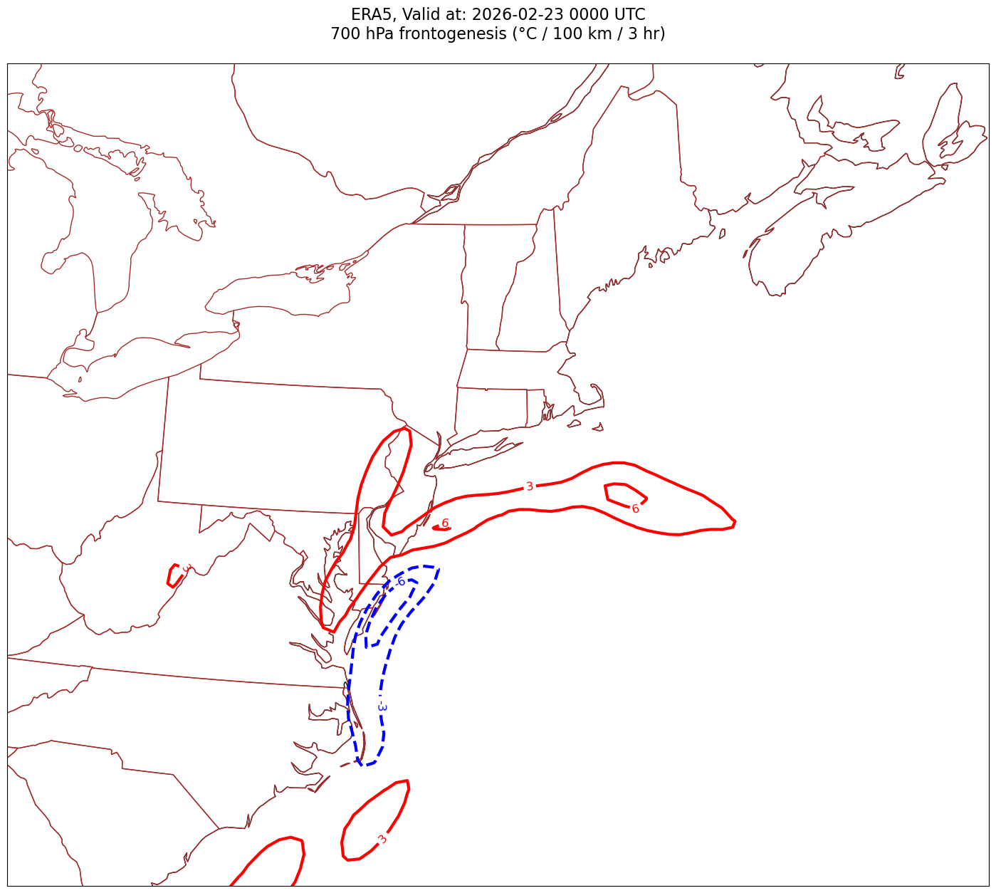
posFrntContours = np.arange (3, 24, frntInc)Now, let’s make our map.
lats = Tp.latitude
lons = Tp.longitude
constrainLat, constrainLon = (0.5, 2.0) # trial and error
for time in dateRange:
print(f'Processing {time}')
# Create the time strings, for the figure title as well as for the file name.
timeStr = dt.strftime(time,format="%Y-%m-%d %H%M UTC")
timeStrFile = dt.strftime(time,format="%Y%m%d%H")
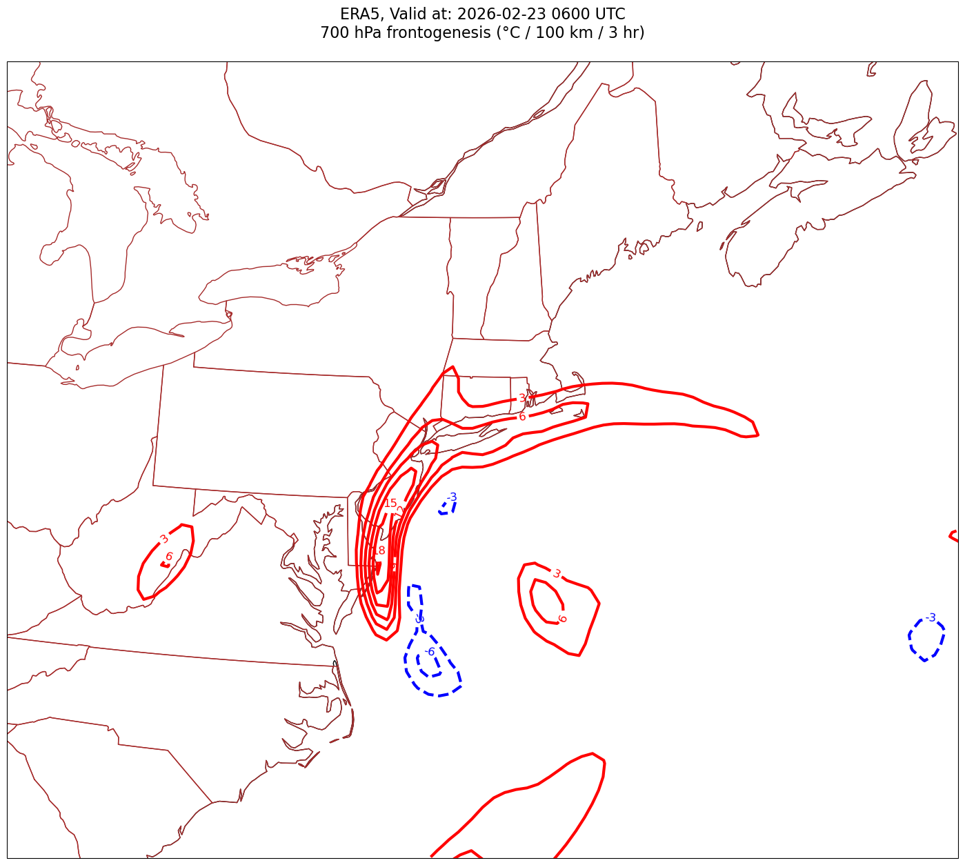
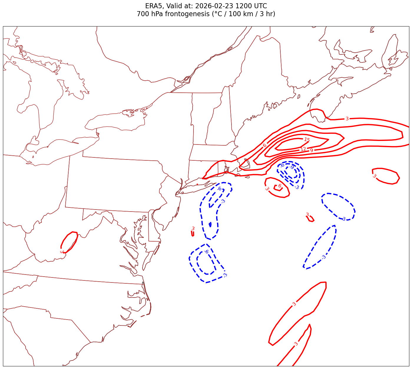
tl1 = f'ERA5, Valid at: {timeStr}'
tl2 = f'{p_level} hPa frontogenesis (°C / 100 km / 3 hr)'
title_line = f'{tl1}\n{tl2}\n'
fig = plt.figure(figsize=(21,15)) # Increase size to adjust for the constrained lats/lons
ax = fig.add_subplot(1,1,1,projection=proj_map)
ax.set_extent ([lonW+constrainLon,lonE-constrainLon,latS+constrainLat,latN-constrainLat])
ax.add_feature(cfeature.COASTLINE.with_scale(res))
ax.add_feature(cfeature.STATES.with_scale(res),edgecolor='brown')
# Need to use Xarray's sel method here to specify the current time for any DataArray you are plotting.
# 1a. Positive contours of frontogenesis
cPosFrnt = ax.contour(lons, lats, FrntSmth.sel(time=time)*scale, levels=posFrntContours, colors='red', linewidths=3, transform=proj_data)
ax.clabel(cPosFrnt, inline=1, fontsize=12, fmt='%.0f')
# 1b. Negative contours of frontogenesis (i.e. frontolysis)
cPosFrnt = ax.contour(lons, lats, FrntSmth.sel(time=time)*scale, levels=negFrntContours, colors='blue', linewidths=3, transform=proj_data)
ax.clabel(cPosFrnt, inline=1, fontsize=12, fmt='%.0f')
title = ax.set_title(title_line,fontsize=16)
#Generate a string for the file name and save the graphic to your current directory.
fileName = f'{timeStrFile}_ERA5_{p_level}_Frontogenesis.png'
fig.savefig(fileName)
Processing 2026-02-23 00:00:00
Processing 2026-02-23 06:00:00
Processing 2026-02-23 12:00:00
What’s next?
Now, create your own plots, based on this and the other diagnostic notebooks we have demonstrated!