Pandas Notebook 1, ATM350 Spring 2026
Here, we read in a text file that has climatological data compiled at the National Weather Service in Albany NY for 2025, previously downloaded and reformatted from the xmACIS2 climate data portal.
We will use the Pandas library to read and analyze the data. We will also use the Matplotlib package to visualize it.
Motivating Science Questions:
How can we analyze and display tabular climate data for a site?
What was the yearly trace of max/min temperatures for Albany, NY last year?
What was the most common 10-degree maximum temperature range for Albany, NY last year?
# import Pandas and Numpy, and use their conventional two-letter abbreviations when we
# use methods from these packages. Also, import matplotlib's plotting package, using its
# standard abbreviation.
import pandas as pd
import numpy as np
import matplotlib.pyplot as plt
Specify the location of the file that contains the climo data. Use the linux ls command to verify it exists.
Note that in a Jupyter notebook, we can simply use the ! directive to “call” a Linux command.
Also notice how we refer to a Python variable name when passing it to a Linux command line in this way ... we enclose it in braces!
year = 2025
file = f'/spare11/atm350/common/data/climo_alb_{year}.csv'
! ls -l {file}
-rw-r--r-- 1 ktyle faculty 15156 Mar 2 19:17 /spare11/atm350/common/data/climo_alb_2025.csv
Use pandas’ read_csv method to open the file. Specify that the data is to be read in as strings (not integers nor floating points).
Once this call succeeds, it returns a Pandas Dataframe object which we reference as df
df = pd.read_csv(file, dtype='string')By simply typing the name of the dataframe object, we can get some of its contents to be “pretty-printed” to the notebook!
dfOur dataframe has 365 or 366 rows (corresponding to all the days in the year) and 10 columns that contain data. This is expressed by calling the shape attribute of the dataframe. The first number in the pair is the # of rows, while the second is the # of columns.
df.shape(365, 10)It will be useful to have a variable (more accurately, an object ) that holds the value of the number of rows, and another for the number of columns.
Remember that Python is a language that uses zero-based indexing, so the first value is accessed as element 0, and the second as element 1!
Look at the syntax we use below to print out the (integer) value of nRows ... it’s another example of string formating.
nRows = df.shape[0]
print (f"Number of rows = {nRows}")
Number of rows = 365
Let’s do the same for the # of columns.
nCols = df.shape[1]
print (f"Number of columns = {nCols}")
Number of columns = 10
To access the values in a particular column, we reference it with its column name as a string. The next cell pulls in all values of the year-month-date column, and assigns it to an object of the same name. We could have named the object anything we wanted, not just Date ... but on the right side of the assignment statement, we have to use the exact name of the column.
Print out what this object looks like.
Date = df['DATE']
print (Date)
0 2025-01-01
1 2025-01-02
2 2025-01-03
3 2025-01-04
4 2025-01-05
...
360 2025-12-27
361 2025-12-28
362 2025-12-29
363 2025-12-30
364 2025-12-31
Name: DATE, Length: 365, dtype: string
Each column of a Pandas dataframe is known as a series. It is basically an array of values, each of which has a corresponding row #. By default, row #'s accompanying a Series are numbered consecutively, starting with 0 (since Python’s convention is to use zero-based indexing).
We can reference a particular value, or set of values, of a Series by using array-based notation. Below, let’s print out the first 30 rows of the dates.
print (Date[:30])0 2025-01-01
1 2025-01-02
2 2025-01-03
3 2025-01-04
4 2025-01-05
5 2025-01-06
6 2025-01-07
7 2025-01-08
8 2025-01-09
9 2025-01-10
10 2025-01-11
11 2025-01-12
12 2025-01-13
13 2025-01-14
14 2025-01-15
15 2025-01-16
16 2025-01-17
17 2025-01-18
18 2025-01-19
19 2025-01-20
20 2025-01-21
21 2025-01-22
22 2025-01-23
23 2025-01-24
24 2025-01-25
25 2025-01-26
26 2025-01-27
27 2025-01-28
28 2025-01-29
29 2025-01-30
Name: DATE, dtype: string
Similarly, let’s print out the last, or 364th row (Why is it 364, not 365???)
print(Date[364])2025-12-31
Note that the selection method does not accept a single negative value.For example, the cell below, which basically requests the last row, won’t work!
print(Date[-1])---------------------------------------------------------------------------
ValueError Traceback (most recent call last)
File /knight/jan25/envs/jan26_env/lib/python3.14/site-packages/pandas/core/indexes/range.py:413, in RangeIndex.get_loc(self, key)
412 try:
--> 413 return self._range.index(new_key)
414 except ValueError as err:
ValueError: range.index(x): x not in range
The above exception was the direct cause of the following exception:
KeyError Traceback (most recent call last)
Cell In[11], line 1
----> 1 print(Date[-1])
File /knight/jan25/envs/jan26_env/lib/python3.14/site-packages/pandas/core/series.py:1133, in Series.__getitem__(self, key)
1130 return self._values[key]
1132 elif key_is_scalar:
-> 1133 return self._get_value(key)
1135 # Convert generator to list before going through hashable part
1136 # (We will iterate through the generator there to check for slices)
1137 if is_iterator(key):
File /knight/jan25/envs/jan26_env/lib/python3.14/site-packages/pandas/core/series.py:1249, in Series._get_value(self, label, takeable)
1246 return self._values[label]
1248 # Similar to Index.get_value, but we do not fall back to positional
-> 1249 loc = self.index.get_loc(label)
1251 if is_integer(loc):
1252 return self._values[loc]
File /knight/jan25/envs/jan26_env/lib/python3.14/site-packages/pandas/core/indexes/range.py:415, in RangeIndex.get_loc(self, key)
413 return self._range.index(new_key)
414 except ValueError as err:
--> 415 raise KeyError(key) from err
416 if isinstance(key, Hashable):
417 raise KeyError(key)
KeyError: -1However, using a negative value as part of a slice does work! Let’s output the last nine values of the series:
print(Date[-9:])356 2025-12-23
357 2025-12-24
358 2025-12-25
359 2025-12-26
360 2025-12-27
361 2025-12-28
362 2025-12-29
363 2025-12-30
364 2025-12-31
Name: DATE, dtype: string
# Enter your code below
maxT = df['MAX']
minT = df['MIN']
Click to reveal only AFTER you have tried your own code!
maxT = df['MAX']
minT = df['MIN']
Examine the two newly-defined Series objects.
maxT0 43
1 38
2 35
3 29
4 30
..
360 22
361 32
362 40
363 25
364 29
Name: MAX, Length: 365, dtype: stringminT0 36
1 30
2 25
3 21
4 19
..
360 11
361 5
362 25
363 19
364 20
Name: MIN, Length: 365, dtype: stringLet’s now list all the days that the high temperature was >= 90. Note carefully how we express this test. It will fail!
hotDays = maxT >= 90---------------------------------------------------------------------------
TypeError Traceback (most recent call last)
Cell In[16], line 1
----> 1 hotDays = maxT >= 90
File /knight/jan25/envs/jan26_env/lib/python3.14/site-packages/pandas/core/ops/common.py:76, in _unpack_zerodim_and_defer.<locals>.new_method(self, other)
72 return NotImplemented
74 other = item_from_zerodim(other)
---> 76 return method(self, other)
File /knight/jan25/envs/jan26_env/lib/python3.14/site-packages/pandas/core/arraylike.py:60, in OpsMixin.__ge__(self, other)
58 @unpack_zerodim_and_defer("__ge__")
59 def __ge__(self, other):
---> 60 return self._cmp_method(other, operator.ge)
File /knight/jan25/envs/jan26_env/lib/python3.14/site-packages/pandas/core/series.py:6138, in Series._cmp_method(self, other, op)
6135 lvalues = self._values
6136 rvalues = extract_array(other, extract_numpy=True, extract_range=True)
-> 6138 res_values = ops.comparison_op(lvalues, rvalues, op)
6140 return self._construct_result(res_values, name=res_name)
File /knight/jan25/envs/jan26_env/lib/python3.14/site-packages/pandas/core/ops/array_ops.py:330, in comparison_op(left, right, op)
321 raise ValueError(
322 "Lengths must match to compare", lvalues.shape, rvalues.shape
323 )
325 if should_extension_dispatch(lvalues, rvalues) or (
326 (isinstance(rvalues, (Timedelta, BaseOffset, Timestamp)) or right is NaT)
327 and lvalues.dtype != object
328 ):
329 # Call the method on lvalues
--> 330 res_values = op(lvalues, rvalues)
332 elif is_scalar(rvalues) and isna(rvalues): # TODO: but not pd.NA?
333 # numpy does not like comparisons vs None
334 if op is operator.ne:
File /knight/jan25/envs/jan26_env/lib/python3.14/site-packages/pandas/core/ops/common.py:76, in _unpack_zerodim_and_defer.<locals>.new_method(self, other)
72 return NotImplemented
74 other = item_from_zerodim(other)
---> 76 return method(self, other)
File /knight/jan25/envs/jan26_env/lib/python3.14/site-packages/pandas/core/arraylike.py:60, in OpsMixin.__ge__(self, other)
58 @unpack_zerodim_and_defer("__ge__")
59 def __ge__(self, other):
---> 60 return self._cmp_method(other, operator.ge)
File /knight/jan25/envs/jan26_env/lib/python3.14/site-packages/pandas/core/arrays/string_.py:1100, in StringArray._cmp_method(self, other, op)
1097 else:
1098 # logical
1099 result = np.zeros(len(self._ndarray), dtype="bool")
-> 1100 result[valid] = op(self._ndarray[valid], other)
1101 res_arr = BooleanArray(result, mask)
1102 if self.dtype.na_value is np.nan:
TypeError: '>=' not supported between instances of 'str' and 'int'Why did it fail? Remember, when we read in the file, we had Pandas assign the type of every column to string! We need to change the type of maxT to a numerical value. Let’s use a 32-bit floating point #, as that will be more than enough precision for this type of measurement. We’ll do the same for the minimum temp.
maxT = maxT.astype("float32")
minT = minT.astype("float32")maxT0 43.0
1 38.0
2 35.0
3 29.0
4 30.0
...
360 22.0
361 32.0
362 40.0
363 25.0
364 29.0
Name: MAX, Length: 365, dtype: float32hotDays = maxT >= 90Now, the test works. What does this data series look like? It actually is a table of booleans ... i.e., true/false values.
print (hotDays)0 False
1 False
2 False
3 False
4 False
...
360 False
361 False
362 False
363 False
364 False
Name: MAX, Length: 365, dtype: bool
As the default output only includes the first and last 5 rows , let’s slice and pull out a period in the middle of the year, where we might be more likely to get some Trues!
print (hotDays[180:195])180 False
181 True
182 False
183 False
184 False
185 False
186 True
187 False
188 False
189 False
190 False
191 False
192 False
193 False
194 False
Name: MAX, dtype: bool
hotDays, as defined above, is Pandas series. We can treat it the same as an existing column in the original dataframe. By passing it into the dataframe, it returns a new DataFrame, which contains only those rows that match the criterion.
df[hotDays]Then, recall that to get a count of the # of rows, we take the first (0th) element of the array returned by a call to the shape method.
Determine the number of days exceeding the specified criterion, and then print out an informative sentence.
n90Max = df[hotDays].shape[0]
print (f'There were {n90Max} days where the high temperature was at least 90°F')
There were 18 days where the high temperature was at least 90°F
Let’s reverse the sense of the test, and get its count. The two counts should add up to the total number of days in the year!
df[maxT < 90].shape[0]347We can combine a test of two different thresholds. Let’s get a count of days where the max. temperature was in the 70s or 80s.
df[(maxT< 90) & (maxT>=70)].shape[0]127Let’s show all the climate data for all these “pleasantly warm” days!
pleasant = df[(maxT< 90) & (maxT>=70)] # Assign the result (a DataFrame) to its own object.
pleasantNotice that after a certain point, not all the rows are displayed to the notebook. We can eliminate the limit of maximum rows and thus show all of the matching days.
pd.set_option ('display.max_rows', None)
pleasantWe can reset this option back to the default.
pd.reset_option('display.max_rows')
pleasantNow let’s visualize the temperature trace over the year! Pandas has a method that directly calls Matplotlib’s plotting package.
maxT.plot()<Axes: >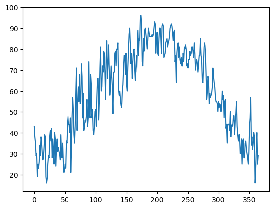
minT.plot()<Axes: >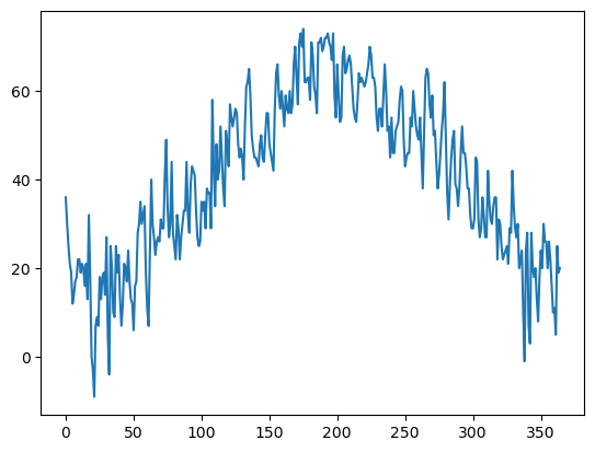
The data plotted fine, but the look could be better. First, let’s import a package, seaborn, that when imported and set using its own method, makes matplotlib’s graphs look better.
Info on seaborn: https://
import seaborn as sns
sns.set()maxT.plot()<Axes: >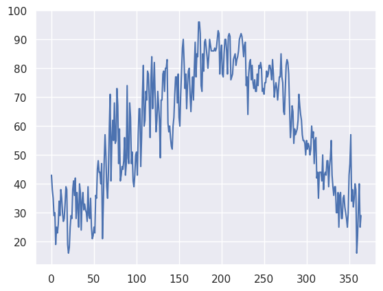
minT.plot()<Axes: >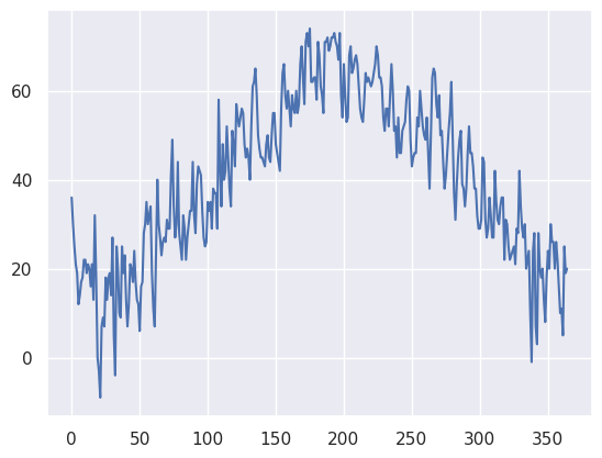
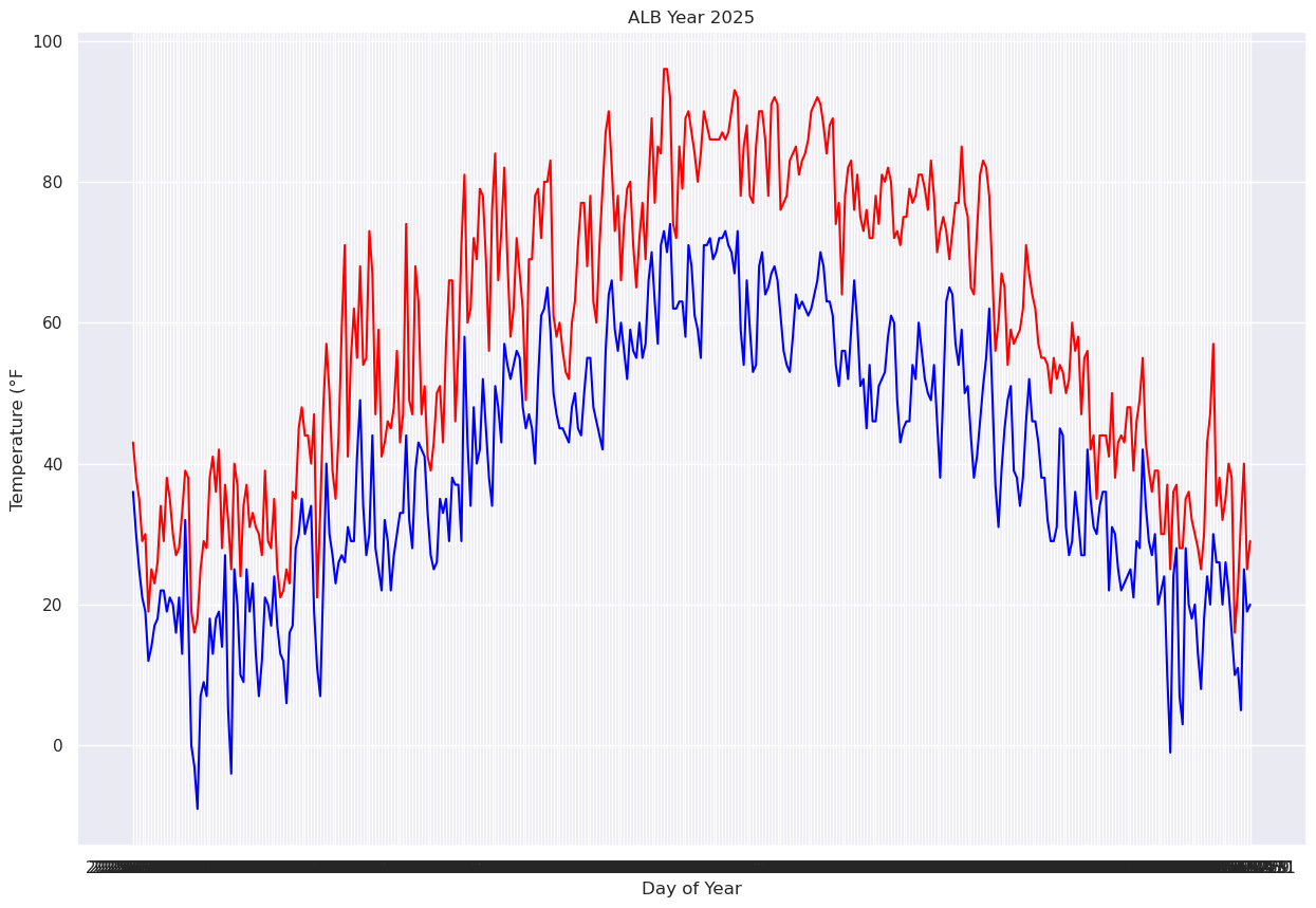
Next, let’s plot the two traces simultaneously on the graph so we can better discern max and min temps (this will also enure a single y-axis that will encompass the range of temperature values). We’ll also add some helpful labels and expand the size of the figure.
You might notice that this graphic did not instantly render. Note that the x-axis label is virtually unreadable. This is because every date is being printed along it!
fig, ax = plt.subplots(figsize=(15,10))
ax.plot (Date, maxT, color='red')
ax.plot (Date, minT, color='blue')
ax.set_title (f"ALB Year {year}")
ax.set_xlabel('Day of Year')
ax.set_ylabel('Temperature (°F')
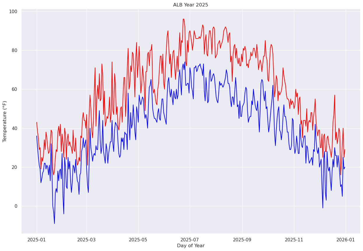
We will deal with this by using one of Pandas’ methods that take strings and convert them to a special type of data ... not strings nor numbers, but datetime objects. Note carefully how we do this here ... it is not terribly intuitive, but we’ll explain it more in an upcoming lecture/notebook on datetime. You will see though that the output column now looks a bit more date-like, with a four-digit year followed by two-digit month and date.
Date = pd.to_datetime(Date,format="%Y-%m-%d")
Date
0 2025-01-01
1 2025-01-02
2 2025-01-03
3 2025-01-04
4 2025-01-05
...
360 2025-12-27
361 2025-12-28
362 2025-12-29
363 2025-12-30
364 2025-12-31
Name: DATE, Length: 365, dtype: datetime64[ns]Matplotlib will recognize this array as being date/time-related, and when we pass it in as the x-axis, the graphic appears faster, and we also have a more meaningful x-axis label.
fig, ax = plt.subplots(figsize=(15,10))
ax.plot (Date, maxT, color='red')
ax.plot (Date, minT, color='blue')
ax.set_title (f"ALB Year {year}")
ax.set_xlabel('Day of Year')
ax.set_ylabel('Temperature (°F)')
We’ll further refine the look of the plot by adding a legend and have vertical grid lines on a frequency of one month.
from matplotlib.dates import DateFormatter, AutoDateLocator,HourLocator,DayLocator,MonthLocatorfig, ax = plt.subplots(figsize=(15,10))
ax.plot (Date, maxT, color='red',label = "Max T")
ax.plot (Date, minT, color='blue', label = "Min T")
ax.set_title (f"ALB Year {year}")
ax.set_xlabel('Date')
ax.set_ylabel('Temperature (°F)' )
ax.xaxis.set_major_locator(MonthLocator(interval=1))
dateFmt = DateFormatter('%b %d')
ax.xaxis.set_major_formatter(dateFmt)
ax.legend (loc="best")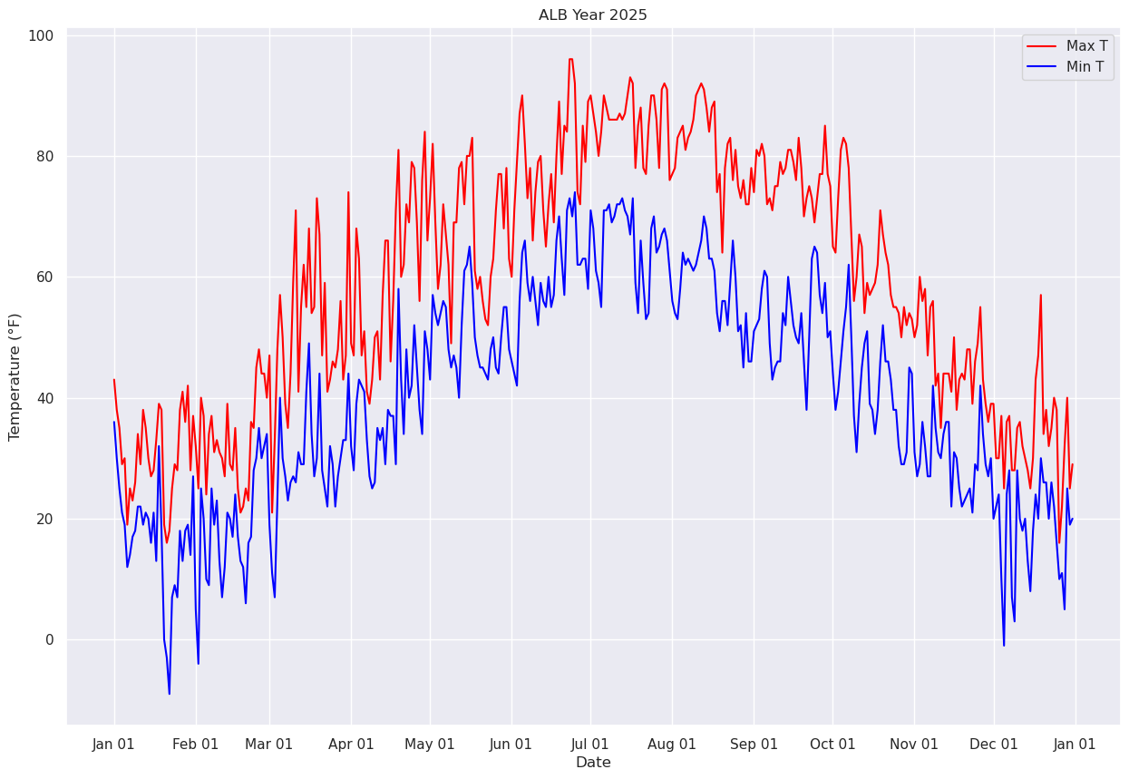
Let’s save our beautiful graphic to disk.
fig.savefig (f'albTemps{year}.png')Now, let’s answer the question, “what was the most common range of maximum temperatures last year in Albany?” via a histogram. We use matplotlib’s hist method.
# Create a figure with a single Axes, and then specify the size of the Axes.
fig, ax = plt.subplots(figsize=(15,10))
# Create a histogram of our data series and divide it in to 10 bins.
ax.hist(maxT, bins=10, color='k', alpha=0.3)
(array([11., 33., 43., 40., 32., 36., 33., 63., 49., 25.]),
 array([16., 24., 32., 40., 48., 56., 64., 72., 80., 88., 96.]),
 <BarContainer object of 10 artists>)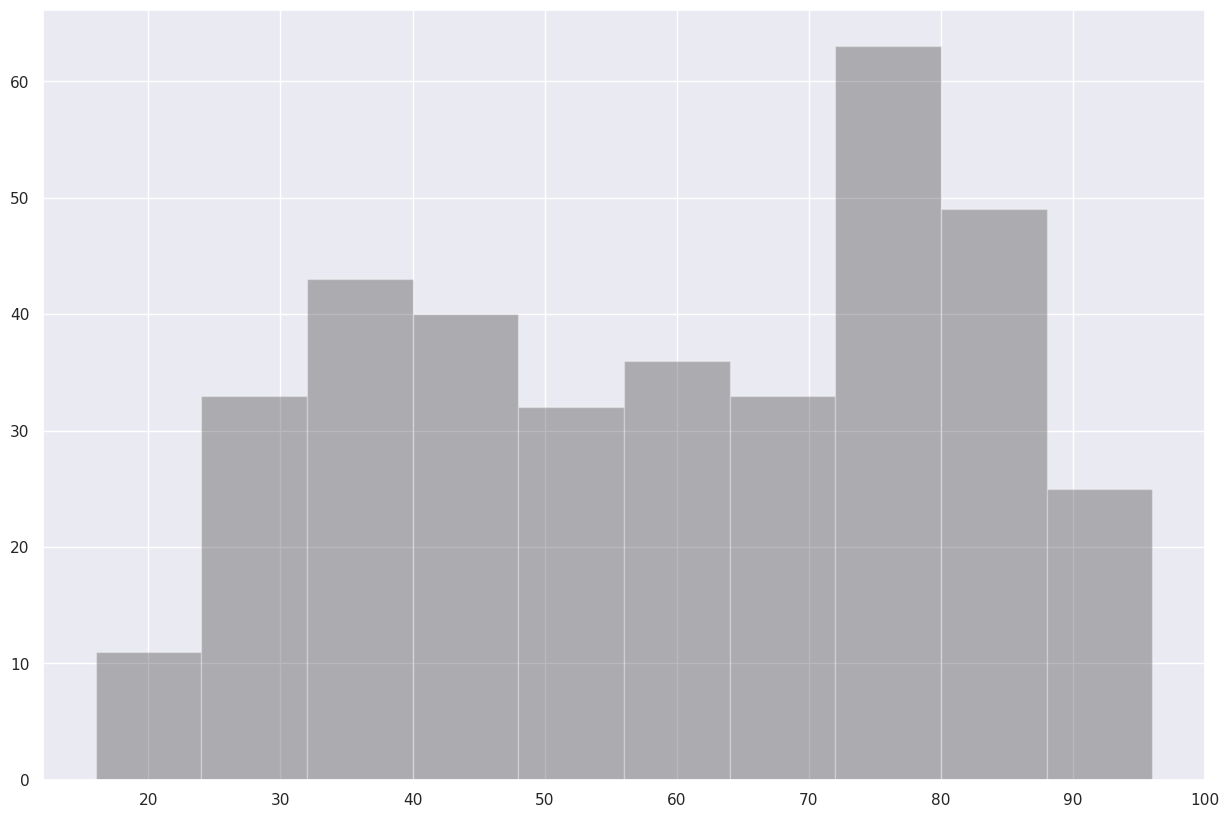
Just about perfect ... except it would be nice to label every ten degrees on the x-axis. This will require two tweaks to the code cell.
First, we pass an additional argument to ax.hist.
ax.hist?Thus, we’ll add bins=10 to the ax.hist function call.
Secondly, to properly label the x-axis, we’ll add a method from another Matplotlib class ... Locator. From Matplotlib’s documentation,
A useful semi-automatic tick locator is MultipleLocator. It is initialized with a base, e.g., 10,
and it picks axis limits and ticks that are multiples of that base.
So let’s import the MultipleLocator method, and specify that each x-axis tick mark and label should occur with x-axis array values that are multiples of 10.
from matplotlib.ticker import MultipleLocator
fig, ax = plt.subplots(figsize=(15,10))
ax.hist(maxT, bins=(0,10,20,30,40,50,60,70,80,90,100), color='k', alpha=0.3)
ax.xaxis.set_major_locator(MultipleLocator(10))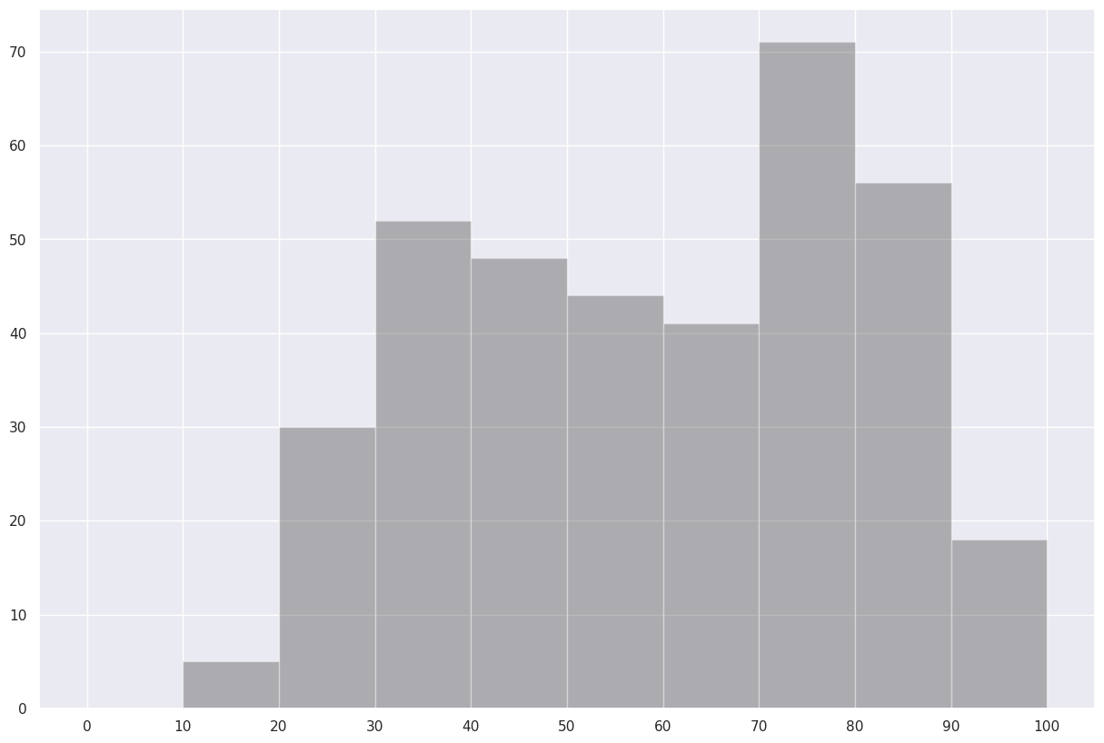
Save this histogram to disk.
fig.savefig("maxT_hist.png")Use the describe method on the maximum temperature series to reveal some simple statistical properties.
maxT.describe()count 365.000000
mean 59.120548
std 20.885399
min 16.000000
25% 41.000000
50% 60.000000
75% 78.000000
max 96.000000
Name: MAX, dtype: float64What’s next?
We will further explore the annual Albany climate dataset with Pandas.