02_Xarray: Large ERA5 archive

Overview¶

Work with a a large ERA5 dataset
Subset the dataset
Select a variable from the dataset
Create a contour line plot of sea-level pressure

Imports¶

import xarray as xr
import pandas as pd
import numpy as np
from metpy.units import units
import metpy.calc as mpcalc
import cartopy.crs as ccrs
import cartopy.feature as cfeature
import matplotlib.pyplot as plt
from datetime import datetime as dt

Work with an Xarray `Dataset`¶

An Xarray Dataset consists of one or more DataArrays. Let’s work with ERA5 data once again, but this time, we will select grids from one of two much larger ERA5 repositories.

# Date/Time specification
Year = 2026
Month = 2
Day = 23
Hour = 0
Minute = 0
dateTime = dt(Year,Month,Day, Hour, Minute)
timeStr = dateTime.strftime("%Y-%m-%d %H%M UTC")

Work with a cloud-served as well as a local ERA5 archive¶

A team at Google Research & Cloud have made some of the ECMWF Reanalysis version 5 (aka ERA-5) accessible in an Analysis Ready, Cloud Optimized (aka ARCO) format.

Access the ERA-5 ARCO, aka WeatherBench2 catalog.

The ERA5 archive runs from 1/1/1959 through 1/10/2023. For dates subsequent to the end-date, we’ll instead load a local archive.

endDate = dt(2023,1,10)
if (dateTime <= endDate): # Use WeatherBench archive

    cloud_source = True
    ds = xr.open_dataset(
     'gs://weatherbench2/datasets/era5/1959-2023_01_10-wb13-6h-1440x721.zarr', 
     chunks={'time': 48},
     consolidated=True,
     engine='zarr'
    )
    # Rename the variable names in this dataset so they use their corresponding short_name attributes
    # Construct a dictionary whose keys are the original variable names, and whose values are their 
    # short names
    
    rename_data_vars = {}
    seen_short_names = set()
    
    for var_name in ds.data_vars:
        short = ds[var_name].attrs.get("short_name")
        # Only rename if:
        # 1. short_name exists
        # 2. We haven't already used it
        if short and short not in seen_short_names:
            rename_data_vars[var_name] = short
            seen_short_names.add(short)
    # Apply renaming
    ds = ds.rename(rename_data_vars)

else: # Use local archive
    import glob, os
    cloud_source = False
    input_directory = '/free/ktyle/era5'
    files = glob.glob(os.path.join(input_directory,'*_era5.nc'))
    ds = xr.open_mfdataset(files,coords='minimal',compat='override')
    # Rename two of the coordinate variables so they match what is in the WeatherBench archive
    ds = ds.rename({'valid_time': 'time', 'pressure_level': 'level'})

Examine the dataset

ds

One attribute of a dataset is its size. We can access that via its nbytes attribute.

print (f'Size of dataset: {ds.nbytes / 1e12} TB')

Size of dataset: 1.694341363896 TB

Define our region of interest; create Cartopy map projection objects for the native dataset as well as what the map will use; select what vertical level we are interested in; and then subset the `Dataset`.¶

latN = 55
latS = 20
lonW = -105
lonE = -55

cLon = (lonW + lonE ) / 2
cLat = (latS + latN ) / 2

# Recall that in ERA5, longitudes run between 0 and 360, not -180 and 180
if (lonW < 0 ):
    lonW = lonW + 360
if (lonE < 0 ):
    lonE = lonE + 360
    
expand_lat = 1
expand_lon = 1

lat_range = np.arange(latS - expand_lat,latN + expand_lat,.5) # expand the data range a bit beyond the plot range

lon_range = np.arange((lonW - expand_lon),(lonE + expand_lon),.5) 

proj_data = ccrs.PlateCarree() # Our data is lat-lon; thus its native projection is Plate Carree.
proj_map = ccrs.LambertConformal(central_longitude=cLon, central_latitude=cLat) # Map projection
res = '50m'

# Select a pressure surface (for ERA5, they are in units of hPa)
p_level = 500

Subset the dataset spatially and temporally.

ds_sub = ds.sel(time=dateTime, level=p_level, latitude=lat_range, longitude=lon_range)

What is the size of this subsetted dataset?

print (f'Size of full dataset: {ds.nbytes / 1e12} TB')
print (f'Size of subsetted dataset: {ds_sub.nbytes / 1e12} TB ({ds_sub.nbytes/1e6} ) MB')

Size of full dataset: 1.694341363896 TB
Size of subsetted dataset: 4.3244e-07 TB (0.43244 ) MB

ds_sub

Data variables selection and subsetting¶

We’ll one data variable (i.e. DataArray), sea-level pressure (msl), from the subsetted Dataset.

slp = ds_sub['msl']

Create a contour plot of gridded data¶

We got a quick plot in the previous notebook. Let’s now customize the map, and focus on a particular region. We will use Cartopy and Matplotlib to plot our SLP contours. Matplotlib has two contour methods:

We will draw contour lines in hPa, with a contour interval of 4.

Now define the range of our contour values and a contour interval. 4 hPa is standard for a sea-level pressure map on a synoptic-scale region.¶

minVal = 900
maxVal = 1076
slp_cint = 4
slp_cintervals = np.arange(minVal, maxVal, slp_cint)
slp_cintervals

array([ 900,  904,  908,  912,  916,  920,  924,  928,  932,  936,  940,
        944,  948,  952,  956,  960,  964,  968,  972,  976,  980,  984,
        988,  992,  996, 1000, 1004, 1008, 1012, 1016, 1020, 1024, 1028,
       1032, 1036, 1040, 1044, 1048, 1052, 1056, 1060, 1064, 1068, 1072])

Matplotlib’s contour methods require three arrays to be passed to them ... x- and y- arrays (longitude and latitude in our case), and a 2-d array (corresponding to x- and y-) of our data variable. So we need to extract the latitude and longitude coordinate variables from our DataArray. We’ll also extract the third coordinate value, time.¶

lats = ds_sub.latitude
lons = ds_sub.longitude
times = ds_sub.time

Note the units are in Pascals. We will exploit MetPy’s unit conversion library soon, but for now let’s just divide the array by 100.

slp_HPA = slp / 100

We’re set to make our map. After creating our figure, setting the bounds of our map domain, and adding cartographic features, we will plot the contours. We’ll assign the output of the contour method to an object, which will then be used to label the contour lines.¶

fig = plt.figure(figsize=(18,12))
ax = plt.subplot(1,1,1,projection=proj_map)
ax.set_extent ([lonW,lonE,latS,latN], crs=ccrs.PlateCarree())
ax.add_feature(cfeature.COASTLINE.with_scale(res))
ax.add_feature(cfeature.STATES.with_scale(res))
CL = ax.contour(lons,lats,slp_HPA,slp_cintervals,transform=proj_data,linewidths=1.25,colors=['green'])
ax.clabel(CL, inline_spacing=0.2, fontsize=11, fmt='%.0f');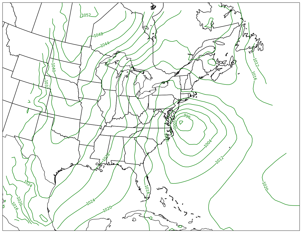

What’s next¶

In the next notebook, we will:

Plot two scalar fields, using contour lines and contour fills
Use MetPy units and calculations
Properly label the figure
Deal with contours not appearing at the western/eastern borders of the plots

References¶

Stern, C., Abernathey, R., Hamman, J., Wegener, R., Lepore, C., Harkins, S., & Merose, A. (2022). Pangeo Forge: Crowdsourcing Analysis-Ready, Cloud Optimized Data Production. Frontiers in Climate, 3. 10.3389/fclim.2021.782909

Overview¶

Imports¶

Work with an Xarray Dataset¶

Work with a cloud-served as well as a local ERA5 archive¶

Define our region of interest; create Cartopy map projection objects for the native dataset as well as what the map will use; select what vertical level we are interested in; and then subset the Dataset.¶

Data variables selection and subsetting¶

Create a contour plot of gridded data¶

Now define the range of our contour values and a contour interval. 4 hPa is standard for a sea-level pressure map on a synoptic-scale region.¶

We’re set to make our map. After creating our figure, setting the bounds of our map domain, and adding cartographic features, we will plot the contours. We’ll assign the output of the contour method to an object, which will then be used to label the contour lines.¶

What’s next¶

Work with an Xarray `Dataset`¶

Define our region of interest; create Cartopy map projection objects for the native dataset as well as what the map will use; select what vertical level we are interested in; and then subset the `Dataset`.¶