03_Xarray: Overlays of variables - ATM 350, Spring 2026

Overview¶

Read two grids from an ERA5 Dataset
Perform unit conversions
Create a well-labeled multi-parameter contour plot of gridded ERA5 data

Imports¶

import xarray as xr
import pandas as pd
import numpy as np
from datetime import datetime as dt
from metpy.units import units
import metpy.calc as mpcalc
import cartopy.crs as ccrs
import cartopy.feature as cfeature
import matplotlib.pyplot as plt

We will repeat the same steps as in the previous notebook, though combined into just a couple cells.

# Date/Time specification
Year = 2021
Month = 2
Day = 23
Hour = 0
Minute = 0
dateTime = dt(Year,Month,Day, Hour, Minute)
timeStr = dateTime.strftime("%Y-%m-%d %H%M UTC")

endDate = dt(2023,1,10)
if (dateTime <= endDate): # Use WeatherBench archive

    cloud_source = True
    ds = xr.open_dataset(
     'gs://weatherbench2/datasets/era5/1959-2023_01_10-wb13-6h-1440x721.zarr', 
     chunks={'time': 48},
     consolidated=True,
     engine='zarr'
)
    # Rename the variable names in this dataset so they use their corresponding short_name attributes
    # Construct a dictionary whose keys are the original variable names, and whose values are their 
    # short names
    
    rename_data_vars = {}
    seen_short_names = set()
    
    for var_name in ds.data_vars:
        short = ds[var_name].attrs.get("short_name")
        # Only rename if:
        # 1. short_name exists
        # 2. We haven't already used it
        if short and short not in seen_short_names:
            rename_data_vars[var_name] = short
            seen_short_names.add(short)
    # Apply renaming
    ds = ds.rename(rename_data_vars)

else: # Use local archive
    import glob, os
    cloud_source = False
    input_directory = '/free/ktyle/era5'
    files = glob.glob(os.path.join(input_directory,'*_era5.nc'))
    ds = xr.open_mfdataset(files,coords='minimal',compat='override')
    # Rename two of the coordinate variables so they match what is in the WeatherBench archive
    ds = ds.rename({'valid_time': 'time', 'pressure_level': 'level'})

latN = 55
latS = 20
lonW = -105
lonE = -55

cLon = (lonW + lonE ) / 2
cLat = (latS + latN ) / 2

# Recall that in ERA5, longitudes run between 0 and 360, not -180 and 180
if (lonW < 0 ):
    lonW = lonW + 360
if (lonE < 0 ):
    lonE = lonE + 360
    
expand_lat = 1
expand_lon = 1

lat_range = np.arange(latS - expand_lat,latN + expand_lat,.5) # expand the data range a bit beyond the plot range

lon_range = np.arange((lonW - expand_lon),(lonE + expand_lon),.5) 


proj_data = ccrs.PlateCarree() # Our data is lat-lon; thus its native projection is Plate Carree.
proj_map = ccrs.LambertConformal(central_longitude=cLon, central_latitude=cLat) # Map projection
res = '50m'

# Select a pressure surface (for ERA5, they are in units of hPa)
p_level = 500

ds_sub = ds.sel(time=dateTime, level=p_level, latitude=lat_range, longitude=lon_range)

slp = ds_sub['msl']

minVal = 900
maxVal = 1076
slp_cint = 4
slp_cintervals = np.arange(minVal, maxVal, slp_cint)

lats = ds_sub.latitude
lons = ds_sub.longitude
times = ds_sub.time

slp_HPA = slp / 100

fig = plt.figure(figsize=(18,12))
ax = fig.add_subplot(1,1,1,projection=proj_map)
ax.set_extent ([lonW,lonE,latS,latN])
ax.add_feature(cfeature.COASTLINE.with_scale(res))
ax.add_feature(cfeature.STATES.with_scale(res))
CL = ax.contour(lons,lats,slp_HPA,slp_cintervals,transform=proj_data,linewidths=1.25,colors=['green'])
ax.clabel(CL, inline_spacing=0.2, fontsize=11, fmt='%.0f');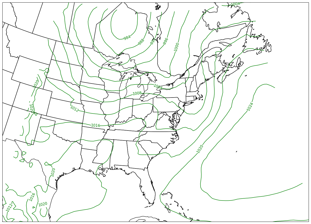

# Write your code here
z = ds_sub['z']

Click to reveal only AFTER you have tried your own code!

z = ds_sub['z']
z

Perform unit conversions¶

Examine the units of slp and z.

slp.units

'Pa'

z.units

'm**2 s**-2'

Convert geopotential to geopotential height in decameters, and Pascals to hectoPascals.

We take the DataArrays and apply MetPy’s unit conversion method.

slp = slp.metpy.convert_units('hPa')
z = mpcalc.geopotential_to_height(z).metpy.convert_units('dam')

slp.nbytes / 1e6, z.nbytes / 1e6 # size in MB for the subsetted DataArrays

(0.030784, 0.030784)

Examine both data arrays after unit conversions. Look at the units attribute now!

slp

Create a well-labeled multi-parameter contour plot of gridded ERA5 reanalysis data¶

We will make contour fills of 500 hPa height in decameters, with a contour interval of 6 dam, and contour lines of SLP in hPa, contour interval = 4.

We’ve already defined the contour intervals for SLP; let’s do the same for geopotential height. 6 dam is standard for 500 hPa.¶

minVal = 474
maxVal = 606
z_cint = 6
z_cintervals = np.arange(minVal, maxVal, z_cint)

Plot the map, with filled contours of 500 hPa geopotential heights, and contour lines of SLP.¶

Create a meaningful title string.

tl1 = f"ERA5 {p_level} hPa heights (dam, filled contours) and SLP (lines, hPa)"
tl2 = f"Valid at: {timeStr}"
title_line = (tl1 + '\n' + tl2 + '\n')

fig = plt.figure(figsize=(18,12))
ax = fig.add_subplot(1,1,1,projection=proj_map)
ax.set_extent ([lonW,lonE,latS,latN], crs=ccrs.PlateCarree())
ax.add_feature(cfeature.COASTLINE.with_scale(res))
ax.add_feature(cfeature.STATES.with_scale(res))
CF = ax.contourf(lons,lats,z, levels=z_cintervals,transform=proj_data,cmap=plt.get_cmap('coolwarm'))
cbar = plt.colorbar(CF,shrink=0.5)
cbar.ax.tick_params(labelsize=16)
cbar.ax.set_ylabel("Height (dam)",fontsize=16)

CL = ax.contour(lons,lats,slp,slp_cintervals,transform=proj_data,linewidths=1.25,colors='green')
ax.clabel(CL, inline_spacing=0.2, fontsize=11, fmt='%.0f')
title = ax.set_title(title_line,fontsize=16)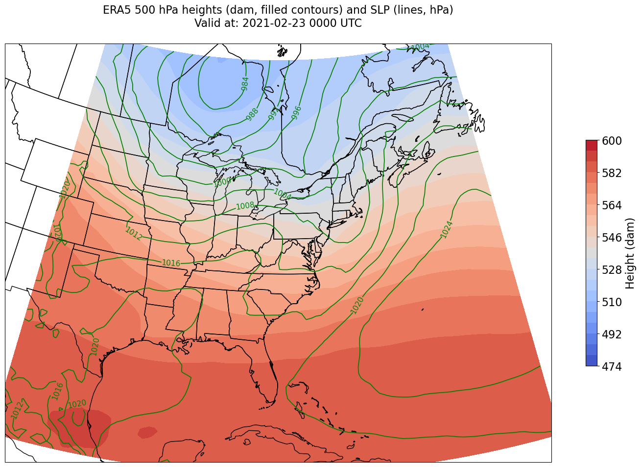

We’re just missing the outer longitudes at higher latitudes. We could do one of two things to resolve this:

Re-subset our original datset by extending the lat/lon rangs (this will require that we edit the relevant cell earlier in the notebook that defined those ranges, followed by re-running all following cells up to this point)
Slightly constrain the map plotting region

Let’s try the latter here.

constrain_lon = 7 # trial and error!
constrain_lat = 2 # trial and error!

fig = plt.figure(figsize=(18,12))
ax = fig.add_subplot(1,1,1,projection=proj_map)
ax.set_extent ([lonW+constrain_lon,lonE-constrain_lon,latS+constrain_lat,latN-constrain_lat], crs=ccrs.PlateCarree())
ax.add_feature(cfeature.COASTLINE.with_scale(res))
ax.add_feature(cfeature.STATES.with_scale(res))
CF = ax.contourf(lons,lats,z, levels=z_cintervals,transform=proj_data,cmap=plt.get_cmap('coolwarm'))
cbar = plt.colorbar(CF,shrink=0.5)
cbar.ax.tick_params(labelsize=16)
cbar.ax.set_ylabel("Height (dam)",fontsize=16)

CL = ax.contour(lons,lats,slp,slp_cintervals,transform=proj_data,linewidths=1.25,colors='green')
ax.clabel(CL, inline_spacing=0.2, fontsize=11, fmt='%.0f')
title = ax.set_title(title_line,fontsize=16);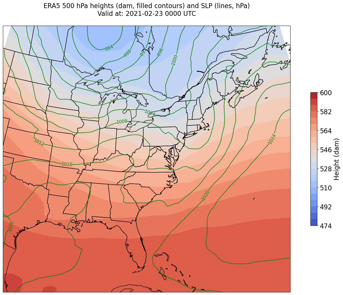

What’s next?¶

We will calculate and visualize diagnostic quantities such as divergence and frontogenesis.