Contextily 2: Other Image Providers

Overview:¶

Explore contextily’s add_basemap function
Access a variety of image sources via the contextily providers object
Plot satellite imagery from NASA

Prerequisites¶

Concepts	Importance	Notes
Contextily 1

Time to learn: 20 minutes

Imports¶

import cartopy.crs as ccrs
import cartopy.feature as cfeature
from metpy.plots import USCOUNTIES
import contextily as ctx
import matplotlib.pyplot as plt

Explore contextily’s `add_basemap` function¶

In our previous notebook, we created a plot with contextily’s default basemap source (Openstreetmaps). Here, we will do the same, over a variety of regions.

Create a Python dictionary that pairs three regions with their corresponding lat-lon boundaries.

extents = {'conus':[-125,-63,23,52],'nys':[-80, -72,40.5,45.2], 'alb':[-73.946,-73.735,42.648,42.707]}
extents

{'conus': [-125, -63, 23, 52],
 'nys': [-80, -72, 40.5, 45.2],
 'alb': [-73.946, -73.735, 42.648, 42.707]}

Note: Python dictionaries are one of the language's core datatypes. Similar to a traditional dictionary, it consists of one or more "words" (termed keys in Python) followed by the corresponding "definitions" (termed values in Python).

Show the keys, followed by the values, of this dictionary.

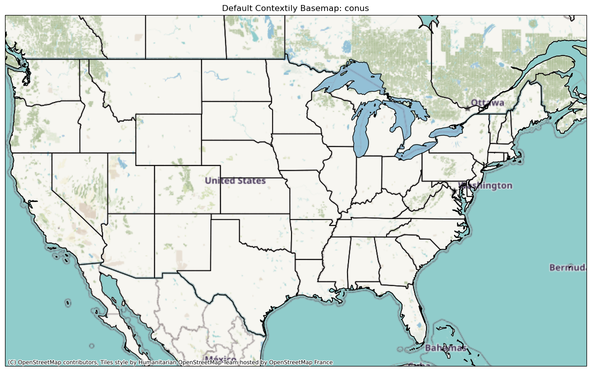
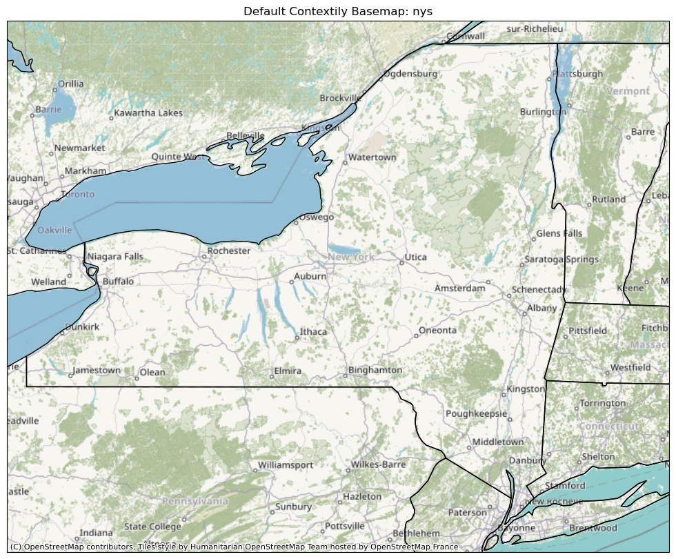
extents.keys()

dict_keys(['conus', 'nys', 'alb'])

extents.values()

dict_values([[-125, -63, 23, 52], [-80, -72, 40.5, 45.2], [-73.946, -73.735, 42.648, 42.707]])

Display the default Contextily basemap for each region.¶

We’ll use what’s called a dictionary comprehension to loop over each region.

for key in extents:
    print(key,extents[key])

    fig = plt.figure(figsize=(15,10))
    ax = plt.axes(projection=ccrs.epsg('3857'))

    res='50m'
    plt.title('Default Contextily Basemap: '+ key)
    ax.coastlines(resolution=res)

    ax.add_feature (cfeature.LAKES.with_scale(res), alpha = 0.5)
    ax.add_feature (cfeature.STATES.with_scale(res))
    ax.set_extent(extents[key], ccrs.PlateCarree())
    ctx.add_basemap(ax)
    plt.show()

conus [-125, -63, 23, 52]

nys [-80, -72, 40.5, 45.2]

alb [-73.946, -73.735, 42.648, 42.707]

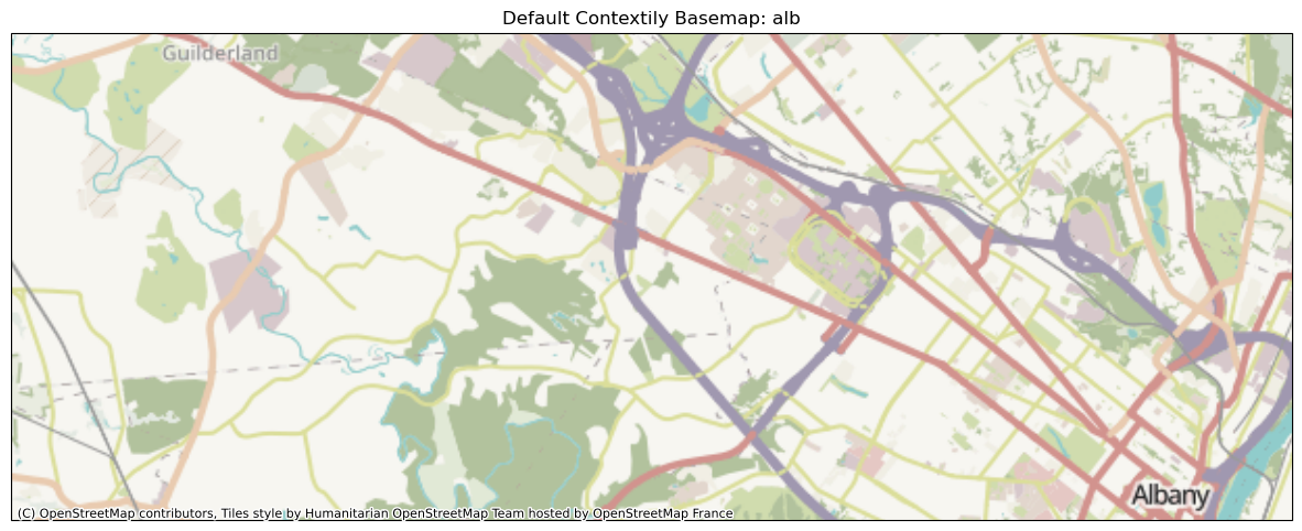
We can see that the same basemap (hosted by OpenStreetMap France) appears, at zoom values automatically determined based on the plotted geographical extent. Notice the street-level resolution for the Albany region.

Access a variety of Contextily’s tile providers.¶

We use Contextily’s providers method. It returns a dictionary. Let’s view that dictionary’s keys:

ctx.providers.keys()

dict_keys(['OpenStreetMap', 'MapTilesAPI', 'OpenSeaMap', 'OPNVKarte', 'OpenTopoMap', 'OpenRailwayMap', 'OpenFireMap', 'SafeCast', 'Stadia', 'Thunderforest', 'BaseMapDE', 'CyclOSM', 'Jawg', 'MapBox', 'MapTiler', 'TomTom', 'Esri', 'OpenWeatherMap', 'HERE', 'HEREv3', 'FreeMapSK', 'MtbMap', 'CartoDB', 'HikeBike', 'BasemapAT', 'nlmaps', 'NASAGIBS', 'NLS', 'JusticeMap', 'GeoportailFrance', 'OneMapSG', 'USGS', 'WaymarkedTrails', 'OpenAIP', 'OpenSnowMap', 'AzureMaps', 'SwissFederalGeoportal', 'TopPlusOpen', 'Gaode', 'Strava', 'OrdnanceSurvey', 'UN'])

Let’s look at a couple of these providers in more detail. First, CartoDB:

ctx.providers.CartoDB

We see that CartoDB has several options itself. For each option, there are several default attributes, such as name and max_zoom.

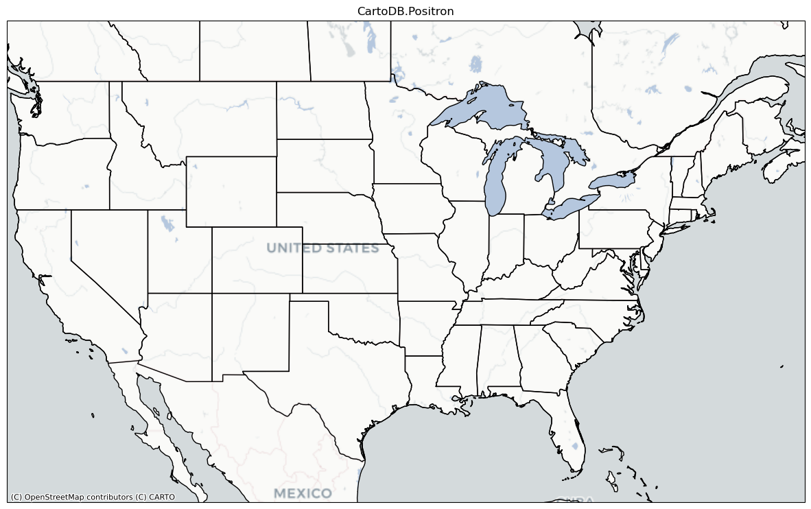
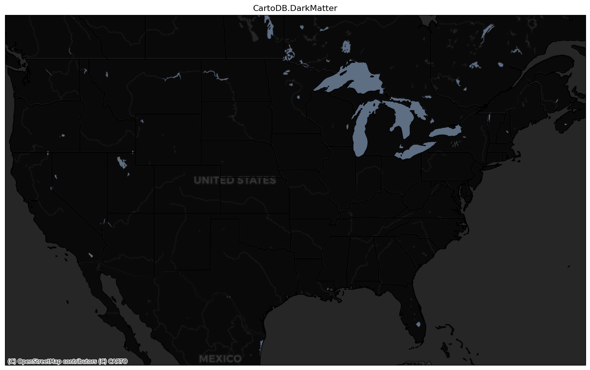
Display two different CartoDB basemaps.¶

We’ll use the source argument for add_basemap via Contextily’s providers object.

bm = {'CartoDB.Positron': ctx.providers.CartoDB.Positron,
      'CartoDB.DarkMatter': ctx.providers.CartoDB.DarkMatter}

for key in bm:
    print (key,bm[key])
    
    fig = plt.figure(figsize=(15,10))
    ax = plt.axes(projection=ccrs.epsg('3857'))

    res='50m'
    plt.title(key)
    ax.coastlines(resolution=res)

    ax.add_feature (cfeature.LAKES.with_scale(res), alpha = 0.5)
    ax.add_feature (cfeature.STATES.with_scale(res))

    ax.set_extent(extents['conus'], ccrs.PlateCarree())
    ctx.add_basemap(ax,source=bm[key])
    plt.show()

CartoDB.Positron {'url': 'https://{s}.basemaps.cartocdn.com/{variant}/{z}/{x}/{y}{r}.png', 'html_attribution': '&copy; <a href="https://www.openstreetmap.org/copyright">OpenStreetMap</a> contributors &copy; <a href="https://carto.com/attributions">CARTO</a>', 'attribution': '(C) OpenStreetMap contributors (C) CARTO', 'subdomains': 'abcd', 'max_zoom': 20, 'variant': 'light_all', 'name': 'CartoDB.Positron'}

CartoDB.DarkMatter {'url': 'https://{s}.basemaps.cartocdn.com/{variant}/{z}/{x}/{y}{r}.png', 'html_attribution': '&copy; <a href="https://www.openstreetmap.org/copyright">OpenStreetMap</a> contributors &copy; <a href="https://carto.com/attributions">CARTO</a>', 'attribution': '(C) OpenStreetMap contributors (C) CARTO', 'subdomains': 'abcd', 'max_zoom': 20, 'variant': 'dark_all', 'name': 'CartoDB.DarkMatter'}

Next, let’s check out NASAGIBS.

Display the 2012 Earth at Night basemap.¶

ctx.providers.NASAGIBS

prov = ctx.providers.NASAGIBS.ViirsEarthAtNight2012
fig = plt.figure(figsize=(15,10))
ax = plt.axes(projection=ccrs.epsg('3857'))

res='50m'
plt.title(prov.name)
ax.coastlines(resolution=res)

ax.add_feature (cfeature.LAKES.with_scale(res), alpha = 0.5)
ax.add_feature (cfeature.STATES.with_scale(res))

ax.set_extent(extents['conus'], ccrs.PlateCarree())
ctx.add_basemap(ax,source=prov)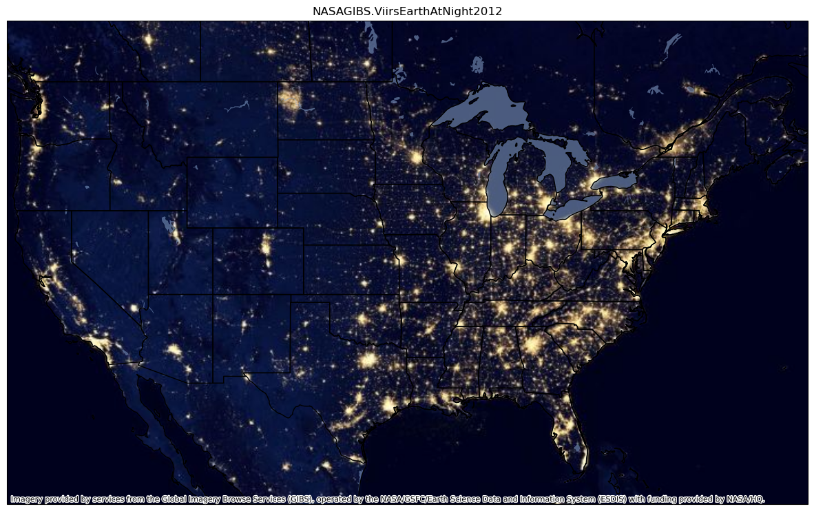

Cool! Now let’s plot the MODIS True Color satellite mosaic.

Plot satellite imagery from NASA’s Modis and Terra satellites.¶

Let’s look specifically at the dictionary corresponding to this satellite product.

ctx.providers.NASAGIBS.ModisTerraTrueColorCR

The time attribute is blank. This product is actually updated once a day, so let’s pick a particular day.

prov = ctx.providers.NASAGIBS.ModisTerraTrueColorCR
fig = plt.figure(figsize=(15,10))
ax = plt.axes(projection=ccrs.epsg('3857'))

time = '2025-10-30'
res='50m'
plt.title(prov.name + ' ' + time)
ax.coastlines(resolution=res)

ax.add_feature (cfeature.LAKES.with_scale(res), alpha = 0.5)
ax.add_feature (cfeature.STATES.with_scale(res))

ax.set_extent(extents['conus'], ccrs.PlateCarree())
ctx.add_basemap(ax,source=prov(time=time))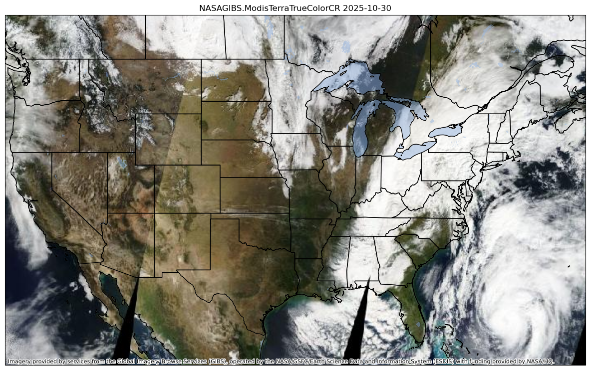

On your own, explore some of the other providers. Some, such as OpenWeatherMap and Mapbox, require you to register for an API key, but have free access plans.