Shapefiles 1: Intro to Shapefiles
Overview:
- Read in the state/province Natural Earth shapefile
- Explore the shapefile using GeoPandas
- Plot the shapefile on a map and overlay with other Natural Earth shapefiles
What is a shapefile?
From Wikipedia:
The shapefile format is a geospatial vector data format for geographic information system (GIS) software. It is developed and regulated by Esri as a mostly open specification for data interoperability among Esri and other GIS software products. The shapefile format can spatially describe vector features: points, lines, and polygons, representing, for example, water wells, rivers, and lakes. Each item usually has attributes that describe it, such as name or temperature.
Imports
import cartopy.crs as ccrs
import cartopy.feature as cfeature
import geopandas as gp
import matplotlib.pyplot as plt
import pandas as pd
import cartopy.io.shapereader as shpreader
from metpy.plots import USCOUNTIES
import glob
import os
Read in a shapefile
Use Cartopy’s shpreader.natural_earth method to read in the highest (10m) resolution states and provinces shapefile.
It will be automatically downloaded if not present, and is cached by default in a hidden subdirectory in your home directory.
res = '10m'
category = 'cultural'
name = 'admin_1_states_provinces'
shpfilename = shpreader.natural_earth(res, category, name)
shpfilenamePosixPath('/home11/staff/ktyle/.local/share/cartopy/shapefiles/natural_earth/cultural/ne_10m_admin_1_states_provinces.shp')What files matching this particular political boundary classification do we have?
path = os.path.dirname(shpfilename)
glob.glob(path + "/ne_10m_admin_1_states_provinces.*")
['/home11/staff/ktyle/.local/share/cartopy/shapefiles/natural_earth/cultural/ne_10m_admin_1_states_provinces.shp',
'/home11/staff/ktyle/.local/share/cartopy/shapefiles/natural_earth/cultural/ne_10m_admin_1_states_provinces.dbf',
'/home11/staff/ktyle/.local/share/cartopy/shapefiles/natural_earth/cultural/ne_10m_admin_1_states_provinces.shx',
'/home11/staff/ktyle/.local/share/cartopy/shapefiles/natural_earth/cultural/ne_10m_admin_1_states_provinces.prj',
'/home11/staff/ktyle/.local/share/cartopy/shapefiles/natural_earth/cultural/ne_10m_admin_1_states_provinces.cpg']We have five files with different suffixes. The first three must be present (see the second reference at the end of the notebook). Here, we will read in the .shp file, using a Pandas-like library, Geopandas, which creates a geo-referenced Pandas Dataframe.
Display all columns in the dataframe. Then create the dataframe and take a look at the first and last five rows (scroll to see all 84 columns).
pd.set_option('display.max_columns', None)
df = gp.read_file(shpfilename)
dfExamine the column names more concisely.
df.columnsIndex(['featurecla', 'scalerank', 'adm1_code', 'diss_me', 'iso_3166_2',
'wikipedia', 'iso_a2', 'adm0_sr', 'name', 'name_alt', 'name_local',
'type', 'type_en', 'code_local', 'code_hasc', 'note', 'hasc_maybe',
'region', 'region_cod', 'provnum_ne', 'gadm_level', 'check_me',
'datarank', 'abbrev', 'postal', 'area_sqkm', 'sameascity', 'labelrank',
'name_len', 'mapcolor9', 'mapcolor13', 'fips', 'fips_alt', 'woe_id',
'woe_label', 'woe_name', 'latitude', 'longitude', 'sov_a3', 'adm0_a3',
'adm0_label', 'admin', 'geonunit', 'gu_a3', 'gn_id', 'gn_name',
'gns_id', 'gns_name', 'gn_level', 'gn_region', 'gn_a1_code',
'region_sub', 'sub_code', 'gns_level', 'gns_lang', 'gns_adm1',
'gns_region', 'min_label', 'max_label', 'min_zoom', 'wikidataid',
'name_ar', 'name_bn', 'name_de', 'name_en', 'name_es', 'name_fr',
'name_el', 'name_hi', 'name_hu', 'name_id', 'name_it', 'name_ja',
'name_ko', 'name_nl', 'name_pl', 'name_pt', 'name_ru', 'name_sv',
'name_tr', 'name_vi', 'name_zh', 'ne_id', 'geometry'],
dtype='object')admin column. We can chain together Pandas` methods such as sort_values and unique to show all of the countries included in the shapefile.df.admin.sort_values().unique()array(['Afghanistan', 'Akrotiri Sovereign Base Area', 'Aland', 'Albania',
'Algeria', 'American Samoa', 'Andorra', 'Angola', 'Anguilla',
'Antarctica', 'Antigua and Barbuda', 'Argentina', 'Armenia',
'Aruba', 'Ashmore and Cartier Islands', 'Australia', 'Austria',
'Azerbaijan', 'Bahrain', 'Bangladesh', 'Barbados',
'Baykonur Cosmodrome', 'Belarus', 'Belgium', 'Belize', 'Benin',
'Bermuda', 'Bhutan', 'Bolivia', 'Bosnia and Herzegovina',
'Botswana', 'Brazil', 'British Indian Ocean Territory',
'British Virgin Islands', 'Brunei', 'Bulgaria', 'Burkina Faso',
'Burundi', 'Cambodia', 'Cameroon', 'Canada', 'Cape Verde',
'Caribbean Netherlands', 'Cayman Islands',
'Central African Republic', 'Chad', 'Chile', 'China',
'Clipperton Island', 'Colombia', 'Comoros', 'Cook Islands',
'Coral Sea Islands', 'Costa Rica', 'Croatia', 'Cuba', 'Curaçao',
'Cyprus', 'Czech Republic', 'Democratic Republic of the Congo',
'Denmark', 'Dhekelia Sovereign Base Area', 'Djibouti', 'Dominica',
'Dominican Republic', 'East Timor', 'Ecuador', 'Egypt',
'El Salvador', 'Equatorial Guinea', 'Eritrea', 'Estonia',
'Ethiopia', 'Falkland Islands', 'Faroe Islands',
'Federated States of Micronesia', 'Fiji', 'Finland', 'France',
'French Polynesia', 'French Southern and Antarctic Lands', 'Gabon',
'Gambia', 'Gaza Strip', 'Georgia', 'Germany', 'Ghana', 'Gibraltar',
'Greece', 'Greenland', 'Grenada', 'Guam', 'Guatemala', 'Guernsey',
'Guinea', 'Guinea Bissau', 'Guyana', 'Haiti',
'Heard Island and McDonald Islands', 'Honduras',
'Hong Kong S.A.R.', 'Hungary', 'Iceland', 'India',
'Indian Ocean Territories', 'Indonesia', 'Iran', 'Iraq', 'Ireland',
'Isle of Man', 'Israel', 'Italy', 'Ivory Coast', 'Jamaica',
'Japan', 'Jersey', 'Jordan', 'Kazakhstan', 'Kenya', 'Kiribati',
'Kosovo', 'Kuwait', 'Kyrgyzstan', 'Laos', 'Latvia', 'Lebanon',
'Lesotho', 'Liberia', 'Libya', 'Liechtenstein', 'Lithuania',
'Luxembourg', 'Macau S.A.R', 'Macedonia', 'Madagascar', 'Malawi',
'Malaysia', 'Maldives', 'Mali', 'Malta', 'Marshall Islands',
'Mauritania', 'Mauritius', 'Mexico', 'Moldova', 'Monaco',
'Mongolia', 'Montenegro', 'Montserrat', 'Morocco', 'Mozambique',
'Myanmar', 'Namibia', 'Nauru', 'Nepal', 'Netherlands',
'New Caledonia', 'New Zealand', 'Nicaragua', 'Niger', 'Nigeria',
'Niue', 'Norfolk Island', 'North Korea', 'Northern Cyprus',
'Northern Mariana Islands', 'Norway', 'Oman', 'Pakistan', 'Palau',
'Panama', 'Papua New Guinea', 'Paraguay', 'Peru', 'Philippines',
'Pitcairn Islands', 'Poland', 'Portugal', 'Puerto Rico', 'Qatar',
'Republic of Serbia', 'Republic of the Congo', 'Romania', 'Russia',
'Rwanda', 'S. Sudan', 'Saint Barthelemy', 'Saint Helena',
'Saint Kitts and Nevis', 'Saint Lucia', 'Saint Martin',
'Saint Pierre and Miquelon', 'Saint Vincent and the Grenadines',
'Samoa', 'San Marino', 'Sao Tome and Principe', 'Saudi Arabia',
'Senegal', 'Seychelles', 'Siachen Glacier', 'Sierra Leone',
'Singapore', 'Sint Maarten', 'Slovakia', 'Slovenia',
'Solomon Islands', 'Somalia', 'Somaliland', 'South Africa',
'South Georgia and the Islands', 'South Korea', 'Spain',
'Spratly Is.', 'Sri Lanka', 'Sudan', 'Suriname', 'Swaziland',
'Sweden', 'Switzerland', 'Syria', 'Taiwan', 'Tajikistan',
'Thailand', 'The Bahamas', 'Togo', 'Tonga', 'Trinidad and Tobago',
'Tunisia', 'Turkey', 'Turkmenistan', 'Turks and Caicos Islands',
'Tuvalu', 'US Naval Base Guantanamo Bay', 'Uganda', 'Ukraine',
'United Arab Emirates', 'United Kingdom',
'United Republic of Tanzania',
'United States Minor Outlying Islands',
'United States Virgin Islands', 'United States of America',
'Uruguay', 'Uzbekistan', 'Vanuatu', 'Vatican', 'Venezuela',
'Vietnam', 'Wallis and Futuna', 'West Bank', 'Western Sahara',
'Yemen', 'Zambia', 'Zimbabwe'], dtype=object)Let’s display all rows that are in the USA.
df.loc[df.admin == 'United States of America']Examine the Geometry column
When Geopandas creates a dataframe from a Shapefile, a key column that gets added is the geometry one. Here we can see that each of the states have Geometry features consisting of Polygons or Multipolygons
df.loc[df.name == 'Colorado']['geometry']3277 POLYGON ((-109.04633 40.99983, -108.88932 40.9...
Name: geometry, dtype: geometrydf.loc[df.name == 'New York']['geometry']1307 MULTIPOLYGON (((-74.69588 44.99803, -74.59611 ...
Name: geometry, dtype: geometryMake a Geopandas dataframe for New York State
dfNYS = df.loc[df.name == 'New York']As with any Pandas Dataframe, we can directly call its plot method for a quick view.
dfNYS.plot(figsize=(12,9))<Axes: >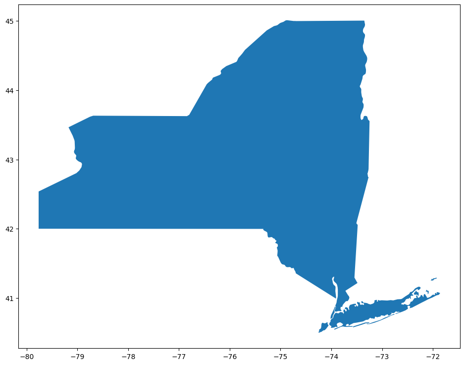
We can create a GeoPandas series consisting only of the Geometry column.
geoNY = df.loc[df.name == 'New York']['geometry']geoNY1307 MULTIPOLYGON (((-74.69588 44.99803, -74.59611 ...
Name: geometry, dtype: geometryExamine the values attribute of this Geopandas geometry object:
geoNY.values<GeometryArray>
[<MULTIPOLYGON (((-74.696 44.998, -74.596 44.998, -74.496 44.999, -74.397 44....>]
Length: 1, dtype: geometryimport cartopy.io.shapereader as shpreader statement.If we take just the first (and only element) of this array, what do we get?
nysPoly = geoNY.values[0]
nysPolyPlot the shapefile
We can now add this object to a Cartopy-referenced Matplotlib plot using Matplotlib’s add_geometries method.
First we’ll comment out all of the Natural Earth shapefiles we typically use. This will produce just a map of NYS.
fig = plt.figure(figsize=(15,10))
ax = plt.axes(projection=ccrs.PlateCarree())
plt.title('NYS')
ax.add_geometries(nysPoly, ccrs.PlateCarree(),
                  edgecolor='black', facecolor='tab:blue', alpha=0.5)
ax.set_extent([-80, -72,40.5,45.2], ccrs.PlateCarree());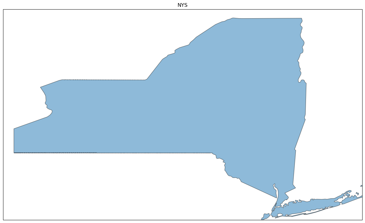
Add additional features to the plot
Now, add some of Cartopy’s Natural Earth features to the plot. We should see that with the exception of the counties (which defaults to a slightly lower resolution (20m) than the others) everything should line up nicely. We’ll slightly expand the map extent so we’ll see neighboring state/province outlines.
res = '10m'
fig = plt.figure(figsize=(15,10))
ax = plt.axes(projection=ccrs.PlateCarree())

plt.title('NYS')
ax.coastlines(resolution=res)
ax.add_geometries(nysPoly, ccrs.PlateCarree(),
                  edgecolor='black', facecolor='tab:blue', alpha=0.5)
ax.add_feature (cfeature.LAKES.with_scale(res), alpha = 0.5)
ax.add_feature (cfeature.STATES.with_scale(res))
ax.add_feature(USCOUNTIES,edgecolor='grey',linewidth=1 );
ax.set_extent([-85, -67,37.5,49.5], ccrs.PlateCarree());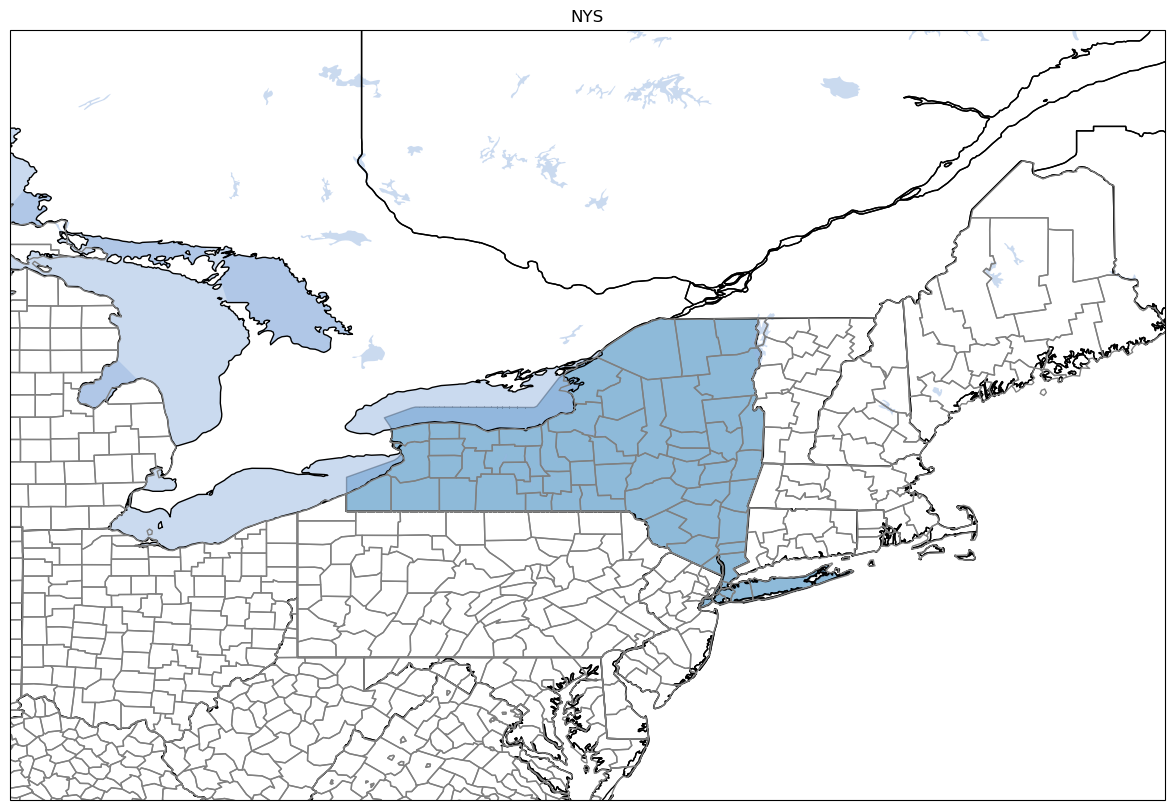
.with_scale('5m') to USCOUNTIES.Summary
- Matplotlib and Cartopy, via the Shapely library, provides support for reading and displaying shapefiles.
- Shapefiles are a form of vector graphics; unlike rasters, they do not degrade as one zooms into them.
- The Geopandas library treats shapefiles as geo-referenced Pandas dataframes.
What’s Next?
We’ll return to cloud-optimized geotiffs, specifically those that are tile-based, with more detail automatically displayed as one zooms in to a particular region.