Rasters 1: Intro to raster data

We’ve already been working with raster data ... namely, with gridded data sets that we’ve used Xarray for analysis.

Overview¶

Access real-time NWP data from Unidata’s THREDDS server
Use Xarray’s plot.imshow to display gridded data as an image
Use Xarray’s open_rasterio method to open and view high-resolution elevation data
Close data objects when you are no longer using them.

Prerequisites¶

Concepts	Importance	Notes
Xarray	Necessary

Time to learn: 15 minutes

Imports¶

import xarray as xr
import rioxarray as rxr
from datetime import datetime, timedelta

Access real-time NWP data from Unidata’s THREDDS server¶

Parse the current time and choose a recent hour when we might expect the model run to be complete. There is normally a ~90 minute lag, but we’ll give it a bit more than that.

now = datetime.now()
year = now.year
month = now.month
day = now.day
hour = now.hour
minute = now.minute
print (year, month, day, hour,minute)

2025 10 21 19 59

# The previous hour's data is typically available shortly after the half-hour, but give it a little extra time 
if (minute < 45): 
    hrDelta = 3
else:
    hrDelta = 2
runTime = now - timedelta(hours=hrDelta)
runTimeStr = runTime.strftime('%Y%m%d %H00 UTC')
modelDate = runTime.strftime('%Y%m%d')
modelHour = runTime.strftime('%H')
modelDay = runTime.strftime('%D')
print (modelDay)
print (modelHour)
print (runTimeStr)

10/21/25
17
20251021 1700 UTC

Create an object pointing to the dataset.

data_url = 'https://thredds.ucar.edu/thredds/dodsC/grib/NCEP/HRRR/CONUS_2p5km/HRRR_CONUS_2p5km_'+ modelDate + '_' + modelHour + '00.grib2'
data_url

'https://thredds.ucar.edu/thredds/dodsC/grib/NCEP/HRRR/CONUS_2p5km/HRRR_CONUS_2p5km_20251021_1700.grib2'

ds = xr.open_dataset(data_url)
xrdSize = ds.nbytes / 1e9
print ("Size of dataset = %.3f GB" % xrdSize)

Size of dataset = 18.136 GB

ds

Tip: This Dataset, while stored in its native (GRIB2) format, presents itself to Xarray as NetCDF. The THREDDS server automatically translates GRIB to NetCDF.
Notice as well that its horizontal dimensions, 2145 x 1377, differs from the HRRR datasets served via cloud providers such as AWS or Google Cloud (1799 x 1099)! The former is a bit higher in horizontal resolution (2.5 km vs 3 km).

Note that the horizontal dimensions of this Dataset are not longitude/latitude. Instead, they represent distances in km from a central origin.

ds.x

ds.y

Use Xarray’s `plot.imshow` to display gridded data as an image¶

One of the output grids is surface pressure. We can visualize it as a proxy for surface elevation.

ds.Pressure_surface

Use Xarray to generate an image, as opposed to a filled contour plot, for the first time in the Dataset.

ds.Pressure_surface.isel(time2=0).plot.imshow(figsize=(15,10))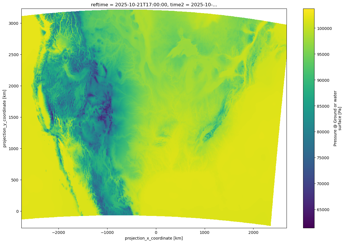

WARNING: A quirk in how a THREDDS data server interprets a GRIB dataset means that the coordinate variable names may change unpredictabily from run to run. In this case, the time dimension was named time. When you run this notebook, the dimension name might also be time, but it could be something else ... such as time1 or time2 Modify the cell above if this occurs. In subsequent notebooks, we'll use a nice **MetPy** utility to dynamically determine the appropriate coordinate variables that accompany an individual variable in an Xarray Dataset.

Tip: Rather than creating filled contours, we have used Xarray's Matplotlib interface to create an image map of surface pressure. Its resolution is the same as the dataset ... in this case, approximately 2.5 km. It fits the definition of what is called raster data.

Note: But there exist other rasterized representations of elevation ... at even higher resolutions ... that are in a particular image format (tiff). Since we never expect these elevations to change (except on very long time scales), we can use these static datasets to complement our visualizations.

Use rioxarray’s `open_rasterio` method to open high-resolution elevation data¶

Natural Earth, the same source that Cartopy utilizes for many of the background features we have used, also provides raster datasets for download. The medium and high-resolution manually-shaded relief files can be accessed from their location in the course data directory.

ds50m = rxr.open_rasterio('/spare11/atm533/data/raster/MSR_50M/MSR_50M.tif')
ds10m = rxr.open_rasterio('/spare11/atm533/data/raster/US_MSR_10M/US_MSR.tif')

Examine these Datasets¶

We now have two Xarray DataArray objects. They are three-dimensional (band, y, and x), with the new dimension called band. There is only one band in each of these data arrays, so we will just pass its one index (0) directly to imshow. Note the horizontal dimemsions ... in both cases, quite a bit higher than the already high-resolution HRRR grid we viewed above. What parts of the world do they represent?

ds10m

ds50m.sel(band=1).plot.imshow(figsize=(15,10))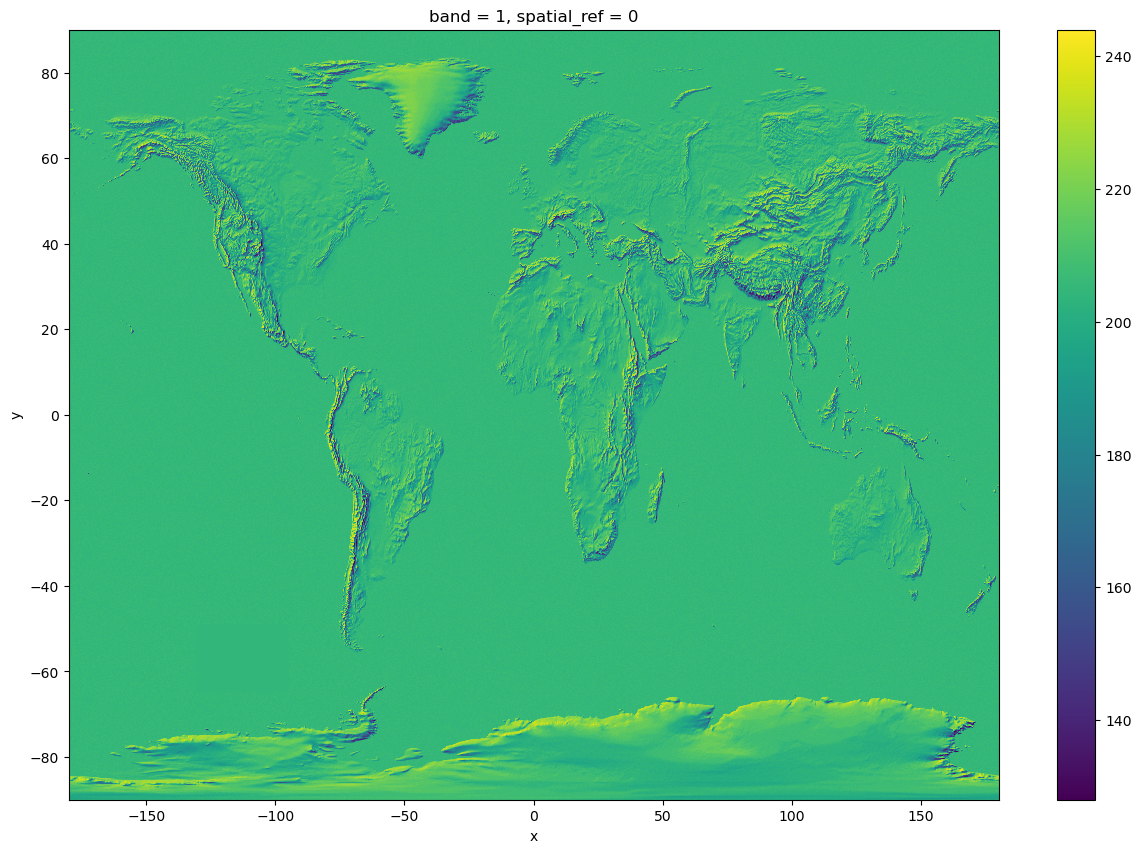

ds10m.sel(band=1).plot.imshow(figsize=(15,10));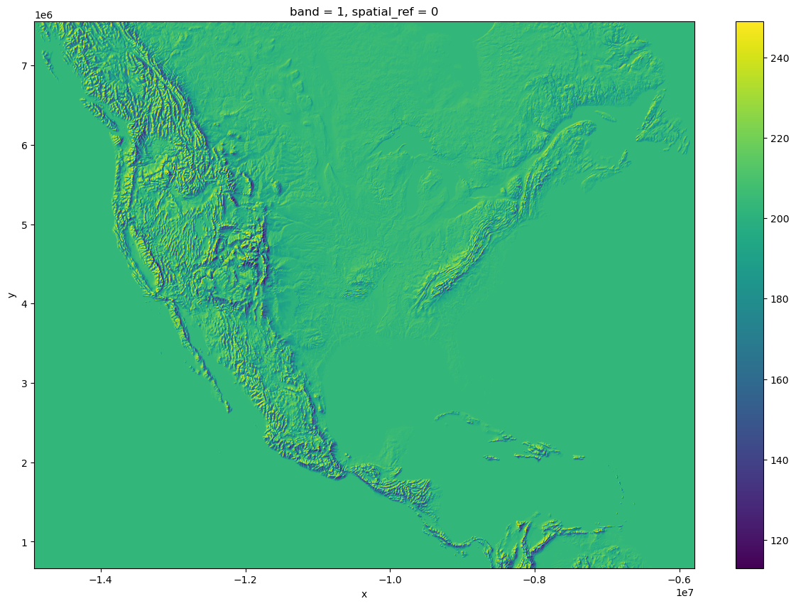

Tip: Notice the x- and y-axis labels. What do you think they represent? Look at the attributes of the spatial_ref coordinate variable for more info.
We'll explore these georeferenced TIFF (tagged image file format) images in more detail in subsequent notebooks!

ds10m.spatial_ref.crs_wkt

'PROJCS["WGS 84 / Pseudo-Mercator",GEOGCS["WGS 84",DATUM["WGS_1984",SPHEROID["WGS 84",6378137,298.257223563,AUTHORITY["EPSG","7030"]],AUTHORITY["EPSG","6326"]],PRIMEM["Greenwich",0,AUTHORITY["EPSG","8901"]],UNIT["degree",0.0174532925199433,AUTHORITY["EPSG","9122"]],AUTHORITY["EPSG","4326"]],PROJECTION["Mercator_1SP"],PARAMETER["central_meridian",0],PARAMETER["scale_factor",1],PARAMETER["false_easting",0],PARAMETER["false_northing",0],UNIT["metre",1,AUTHORITY["EPSG","9001"]],AXIS["Easting",EAST],AXIS["Northing",NORTH],EXTENSION["PROJ4","+proj=merc +a=6378137 +b=6378137 +lat_ts=0 +lon_0=0 +x_0=0 +y_0=0 +k=1 +units=m +nadgrids=@null +wktext +no_defs"],AUTHORITY["EPSG","3857"]]'

Close the file handles so they don’t stay resident in memory.¶

ds.close()
ds10m.close()
ds50m.close()

Summary¶

We can access real-time NWP data via the Unidata THREDDS server
THREDDS automatically translates data in supported formats (such as GRIB) into NetCDF.
Gridded data arrays are a type of raster data.
Matplotlib’s imshow method displays raster data as an image.
A frequently-used image format is tiff.
TIFFS can be geo-referenced, making them very useful in map-based visualizations.