Rasters 2: Overlays

Overview¶

Read in a raster file in GeoTIFF format of surface elevation using the Rioxarray package
Explore the attributes of the GeoTIFF file
Plot the GeoTIFF using Matplotlib and Cartopy
Overlay the GeoTIFF on a plot of realtime forecast reflectivity data

Prerequisites¶

Concepts	Importance	Notes
Rasters 1	Necessary

Time to learn: 30 minutes

WARNING: due to the high-resolutions of both the raster image and the HRRR forecast reflectivity, this notebook will use approx. 8GB of system memory as you run it! You may wish to simply use this already-populated notebook as a reference, and only modify/run through it when you need to.
Be sure to close and shutdown the notebook when finished!

Imports¶

from datetime import datetime, timedelta
import pandas as pd
import matplotlib.pyplot as plt
import cartopy.crs as ccrs
import cartopy.feature as cfeature
import numpy as np
import xarray as xr

from metpy.plots import USCOUNTIES
from metpy.plots import ctables
import rioxarray as rxr
from matplotlib.colors import BoundaryNorm
from matplotlib.ticker import MaxNLocator

Note: Besides the rioxarray library, we've also imported USCOUNTIES from MetPy. This allows for the plotting of US county line boundaries, similar to other Cartopy cartographic features such as states.
Additonally, we've imported a set of color tables, also from MetPy.
We've also imported a couple additional methods from Matplotlib, which we'll use to customize the look of our plot when using the imshow method.

Read in a raster file in GeoTIFF format¶

Process the topography GeoTIFF file, downloaded from Natural Earth, using the rioxarray package. This package provides an xarray interface while also presenting functionality similar to the rasterio library.

msr = rxr.open_rasterio('/spare11/atm533/data/raster/US_MSR_10M/US_MSR.tif')

Explore the GeoTIFF file. Remember, it’s a TIFF file that is georeferenced.

msr

Note: rioxarray returns a DataArray that has a unique coordinate variable, spatial_ref. This coordinate variable's attributes includes CRS info in what's called well-known text (WKT) format, as well as the Affine transformation parameters. See references at the end of this notebook.

Get the bounding box coordinates of the raster file. We will need to pass them to Matplotlib’s imshow function.

left,bottom,right,top = msr.rio.bounds()
left,bottom,right,top

(-14920200.0, 666726.142827049, -5787726.0672549475, 7560000.0)

These values represent the coordinates, in units specific to the GeoTIFF’s geographic coordinate reference system, of the lower-left and upper-right corners of the raster file.

Get the projection info, which we can later use in Cartopy. A rioxarray dataset object has an attribute called crs for this purpose.

msr.rio.crs

CRS.from_wkt('PROJCS["WGS 84 / Pseudo-Mercator",GEOGCS["WGS 84",DATUM["WGS_1984",SPHEROID["WGS 84",6378137,298.257223563,AUTHORITY["EPSG","7030"]],AUTHORITY["EPSG","6326"]],PRIMEM["Greenwich",0,AUTHORITY["EPSG","8901"]],UNIT["degree",0.0174532925199433,AUTHORITY["EPSG","9122"]],AUTHORITY["EPSG","4326"]],PROJECTION["Mercator_1SP"],PARAMETER["central_meridian",0],PARAMETER["scale_factor",1],PARAMETER["false_easting",0],PARAMETER["false_northing",0],UNIT["metre",1,AUTHORITY["EPSG","9001"]],AXIS["Easting",EAST],AXIS["Northing",NORTH],EXTENSION["PROJ4","+proj=merc +a=6378137 +b=6378137 +lat_ts=0 +lon_0=0 +x_0=0 +y_0=0 +k=1 +units=m +nadgrids=@null +wktext +no_defs"],AUTHORITY["EPSG","3857"]]')

Assign this CRS to a Cartopy projection object.

projMSR = ccrs.epsg('3857')

Note: What does this coordinate reference system refer to? It is called Web Mercator, aka Pseudo Mercator, which is what is used in most web-based interactive mapping applications, such as Google Earth. See https://epsg.io/3857

Examine the spatial_ref attribute of this Dataset.

msr.spatial_ref

This information makes it possible for GIS applications, such as Cartopy, to transform data that’s represented in one CRS to another.

Select the first (and only) band and redefine the DataArray object, so it only has dimensions of x and y.

msr = msr.sel(band=1)

Determine the min and max values.

msr.min(),msr.max()

(<xarray.DataArray ()> Size: 1B
 array(113, dtype=uint8)
 Coordinates:
     band         int64 8B 1
     spatial_ref  int64 8B 0,
 <xarray.DataArray ()> Size: 1B
 array(249, dtype=uint8)
 Coordinates:
     band         int64 8B 1
     spatial_ref  int64 8B 0)

Note: For this raster file, the values (which were manually determined by its author) are inversely proportional to elevation. Thus, lower values correspond to higher elevation.

The next cell will determine how the topography field will be displayed on the figure. These settings work well for this dataset, but obviously must be customized for use with other raster images. This is akin to setting contour fill intervals, but instead of using Matplotlib’s contourf method, we will use imshow, and take advantage of the two Matplotlib methods we imported at the start of the notebook.

# Pick a binning (which is analagous to the # of fill contours, and set a min/max range)
levels = MaxNLocator(nbins=30).tick_values(msr.min(), msr.max()-20)

# Pick the desired colormap, sensible levels, and define a normalization
# instance which takes data values and translates those into levels.
# In this case, we take a color map of 256 discrete colors and normalize them down to 30.
cmap = plt.get_cmap('gist_gray')
norm = BoundaryNorm(levels, ncolors=cmap.N, clip=True)

Examine the levels.

levels

array([112., 116., 120., 124., 128., 132., 136., 140., 144., 148., 152.,
       156., 160., 164., 168., 172., 176., 180., 184., 188., 192., 196.,
       200., 204., 208., 212., 216., 220., 224., 228., 232.])

Plot the GeoTIFF using Matplotlib and Cartopy¶

Create a region over which we will plot ... in this case, centered over NY State.

latN_sub = 45.2
latS_sub = 40.2
lonW_sub = -80.0
lonE_sub = -71.5
cLat_sub = (latN_sub + latS_sub)/2.
cLon_sub = (lonW_sub + lonE_sub )/2.

proj_sub = ccrs.LambertConformal(central_longitude=cLon_sub,
                             central_latitude=cLat_sub,
                             standard_parallels=[cLat_sub])

Plot the GeoTIFF using imshow. Just as we’ve previously transformed data from PlateCarree (lat/lon), here we transform from the Web Mercator projection that the elevation raster file uses.

res = '50m' # Use the medium resolution Natural Earth shapefiles so plotting goes a bit faster than with the highest (10m)
fig = plt.figure(figsize=(18,12))
ax = plt.subplot(1,1,1,projection=proj_sub)
ax.set_extent((lonW_sub,lonE_sub,latS_sub,latN_sub),crs=ccrs.PlateCarree())
ax.set_facecolor(cfeature.COLORS['water'])
ax.add_feature (cfeature.LAND.with_scale(res))
ax.add_feature(cfeature.COASTLINE.with_scale(res))
ax.add_feature (cfeature.LAKES.with_scale(res), alpha = 0.5)
ax.add_feature (cfeature.STATES.with_scale(res))
ax.add_feature(USCOUNTIES,edgecolor='grey', linewidth=1 );
im = ax.imshow(msr,cmap=plt.get_cmap('gist_gray'), alpha=0.4,norm=norm,transform=projMSR);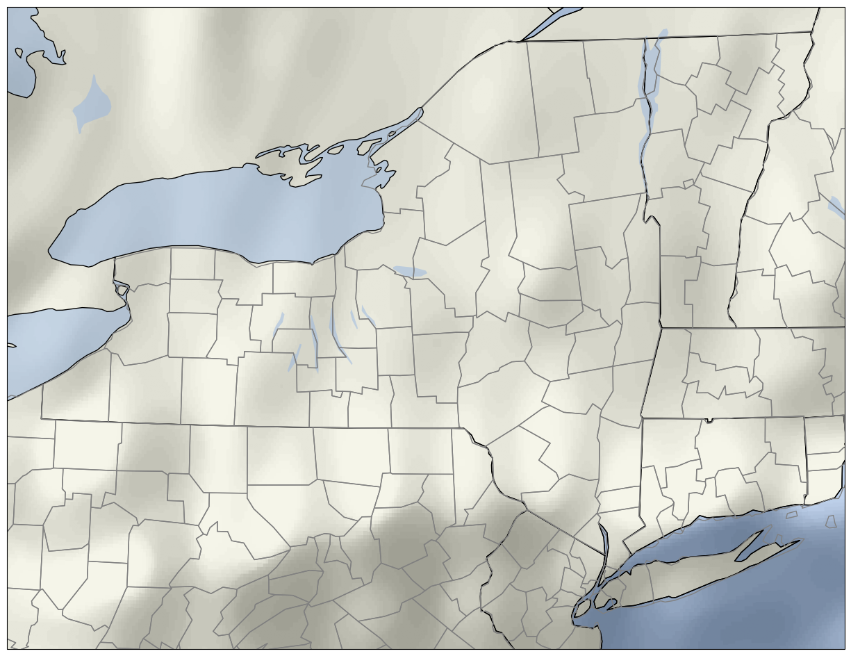

WTF! Well ... that does not seem to accurately represent the topography in the NE US! One additional parameter we must pass into imshow is extent. The default values are not what we want; instead, we use the Bounding Box values that we read in earlier. See the documentation for extent in imshow's documentation.

res = '50m'
fig = plt.figure(figsize=(18,12))
ax = plt.subplot(1,1,1,projection=proj_sub)
ax.set_extent((lonW_sub,lonE_sub,latS_sub,latN_sub),crs=ccrs.PlateCarree())
ax.set_facecolor(cfeature.COLORS['water'])
ax.add_feature (cfeature.LAND.with_scale(res))
ax.add_feature(cfeature.COASTLINE.with_scale(res))
ax.add_feature (cfeature.LAKES.with_scale(res), alpha = 0.5)
ax.add_feature (cfeature.STATES.with_scale(res))
ax.add_feature(USCOUNTIES,edgecolor='grey', linewidth=1)
# Pass in the bounding box coordinates as the value for extent
im = ax.imshow(msr, extent = [left,right,bottom,top],cmap=plt.get_cmap('gist_gray'),
                 alpha=0.4,norm=norm,transform=projMSR);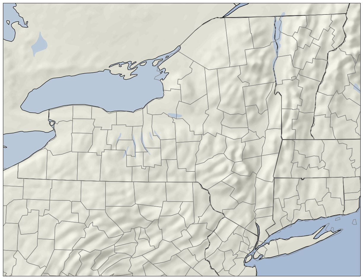

That’s more like it! Now, we can plot maps that include one (or more) GeoTIFF raster images, while also overlaying meteorological data, such as point observations or gridded model output.

Overlay the GeoTIFF on a plot of realtime forecast reflectivity data¶

Below, we go through the same steps that we did in the first Raster notebook to gather the latest HRRR model output, but plot filled contours of forecasted 1km above ground level radar reflectivity over the background of topography. We’ll plot over the CONUS.

now = datetime.now()
year = now.year
month = now.month
day = now.day
hour = now.hour
minute = now.minute
print (year, month, day, hour,minute)

if (minute < 45): 
    hrDelta = 3
else:
    hrDelta = 2
runTime = now - timedelta(hours=hrDelta)
runTimeStr = runTime.strftime('%Y%m%d %H00 UTC')
modelDate = runTime.strftime('%Y%m%d')
modelHour = runTime.strftime('%H')
modelDay = runTime.strftime('%D')
print (modelDay)
print (modelHour)
print (runTimeStr)

2025 10 21 20 0
10/21/25
17
20251021 1700 UTC

data_url = 'https://thredds.ucar.edu/thredds/dodsC/grib/NCEP/HRRR/CONUS_2p5km/HRRR_CONUS_2p5km_'+ modelDate + '_' + modelHour + '00.grib2'

Create an Xarray Dataset and apply MetPy’s [parse_cf] function which, among other things, will ease the determination of the dataset’s map projection, and also ensure that coordinate variables are in SI units (e.g., meters for length and Pascals for pressure).

ds = xr.open_dataset(data_url)
ds = ds.metpy.parse_cf()

ds

Select the 1km AGL reflectivity variable from the Dataset

var = ds.Reflectivity_height_above_ground

Get the DataArray’s map projection

proj_data = var.metpy.cartopy_crs

Examine the reflectivity grid

var

GRIB files that are served by THREDDS are automatically converted into NetCDF. A quirk in this translation can result in certain dimensions (typically those that are time or vertically-based) varying from run-to-run. For example, the time coordinate dimension for a given variable might be time in one run, but time1 (or time2, time3, etc.) in another run. This poses a challenge any time we want to subset a DataArray. For example, if a particular dataset had vertical levels in units of hPa, the dimension name for the geopotential height grid might be isobaric. If we wanted to select only the 500 and 700 hPa levels, we might write the following line of code:

Z = ds.sel(isobaric=[500, 700])

This would fail if we pointed to model output from a different time, and the vertical coordinate name for geopotential height was instead isobaric1.

Via strategic use of Python dictionaries, we can programmatically deal with this!

First, let’s use some MetPy accessors that determine the dimension names for times and vertical levels:

timeDim, vertDim = var.metpy.time.name, var.metpy.vertical.name
timeDim, vertDim

('time2', 'height_above_ground1')

We next construct dictionaries corresponding to each desired subset of the relevant dimensions. Here, we specify the first time, and the one and only vertical level:

idxTime = 0 # First time
idxVert = 0 # First (and in this case, only) vertical level

timeDict = {timeDim: idxTime}
vertDict = {vertDim: idxVert}

timeDict, vertDict

({'time2': 0}, {'height_above_ground1': 0})

We can now pass in these dictionaries to Xarray’s `sel` or `isel` methods.¶

Create a title string for the figure

validTime = var.isel(timeDict)[timeDim].values # Returns validTime as a NumPy Datetime 64 object
validTime = pd.Timestamp(validTime) # Converts validTime to a Pandas Timestamp object
timeStr = validTime.strftime("%Y-%m-%d %H%M UTC") # We can now use Datetime's strftime method to create a time string.
tl1 = "HRRR 1km AGL Reflectivity (dBZ)"
tl2 = str('Valid at: '+ timeStr)
title_line = (tl1 + '\n' + tl2 + '\n')

Select the desired time and vertical level

grid = var.isel(vertDict).isel(timeDict)

Use a set of color tables that mimics what the National Weather Services uses for its reflectivity plots.

ref_norm, ref_cmap = ctables.registry.get_with_steps('NWSReflectivity', 5, 5)

refl_range = np.arange(5,80,5)

Assign objects for the x- and y- arrays.

x = grid.x
y = grid.y

Make the map.

Note:

For speed, choose the coarsest resolution for the cartographic features. It's fine for a larger view such as the CONUS.
For readability, do not plot county outlines for a regional extent as large as the CONUS
This step is particularly memory-intensive, since we are reading in two high-resolution rasters (elevation and reflectivity)!

res = '110m'
fig = plt.figure(figsize=(18,12))
ax = plt.subplot(1,1,1,projection=proj_data)
ax.set_extent((-125,-68,20,52),crs=ccrs.PlateCarree())
ax.set_facecolor(cfeature.COLORS['water'])
ax.add_feature (cfeature.LAND.with_scale(res))
ax.add_feature(cfeature.COASTLINE.with_scale(res))
ax.add_feature (cfeature.LAKES.with_scale(res), alpha = 0.5)
ax.add_feature (cfeature.STATES.with_scale(res))
# Usually avoid plotting counties once the regional extent is large
#ax.add_feature(USCOUNTIES,edgecolor='grey', linewidth=1 );
im = ax.imshow(msr,extent=[left, right, bottom, top],cmap=plt.get_cmap('gist_gray'),
                 alpha=0.4,norm=norm,transform=projMSR)
CF = ax.contourf(x,y,grid,levels=refl_range,cmap=ref_cmap,alpha=0.5,transform=proj_data)
cbar = plt.colorbar(CF,fraction=0.046, pad=0.03,shrink=0.5)
cbar.ax.tick_params(labelsize=10)
cbar.ax.set_ylabel("Reflectivity (dBZ)",fontsize=10);
title = ax.set_title(title_line,fontsize=16)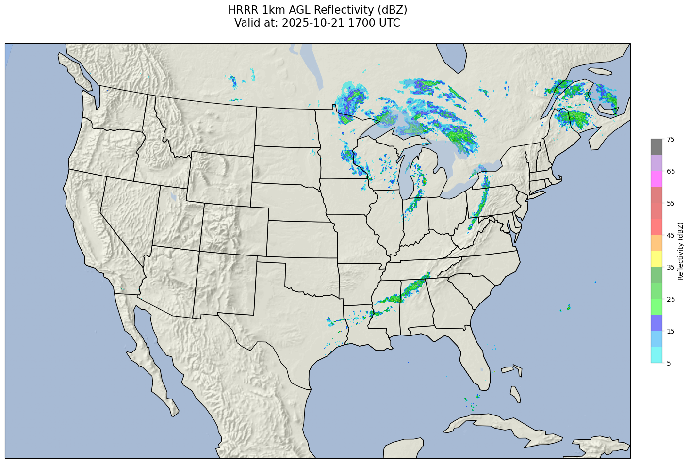

Summary¶

The Rioxarray package allows for raster-specific methods on geo-referenced Xarray objects.
When using imshow with Cartopy’s geo-referenced axes in Matplotlib, one must specify the extent, derived from the GeoTIFF’s bounding box.
GeoTIFFs can be overlayed with other geo-referenced datasets, such as gridded fields or point observations.
The higher the resolution, the higher the memory usage.