Intro to Xarray
Outline
- Introduction to Xarray
- Anatomy of a DataArray
Imports
import xarray as xrWhile Pandas is great for many purposes, extending its inherently 2-d data representation to a multidimensional dataset, such as 4-dimensional (time, vertical level, longitude (x) and latitude (y)) gridded NWP/Climate model output, is unwise.
Gridded data is typically written in a non-ASCII (i.e., not human-readable) format. The two most widely-used formats are GRIB and NetCDF. Another format, quickly gaining traction, is Zarr. These binary formats take up less storage space than text.
The Xarray package is ideally-suited for gridded data, in particular NetCDF and Zarr. It builds and extends on the multi-dimensional data structure in NumPy. We will see that some of the same methods we’ve used for Pandas have analogues in Xarray.
As a a general introduction to Xarray, below is part of a section from the Xarray Tutorial that was presented at the SciPy 2020 conference:
(Start of SciPy 2020 Xarray Tutorial snippet)
Multi-dimensional (a.k.a. N-dimensional, ND) arrays (sometimes called “tensors”) are an essential part of computational science. They are encountered in a wide range of fields, including physics, astronomy, geoscience, bioinformatics, engineering, finance, and deep learning. In Python, NumPy provides the fundamental data structure and API for working with raw ND arrays. However, real-world datasets are usually more than just raw numbers; they have labels which encode information about how the array values map to locations in space, time, etc.
Here is an example of how we might structure a dataset for a weather forecast:
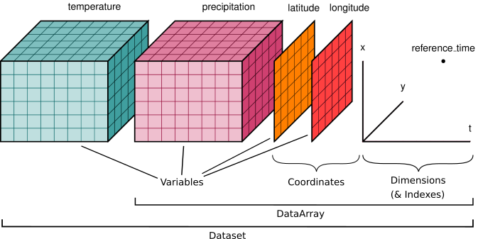
You’ll notice multiple data variables (temperature, precipitation), coordinate variables (latitude, longitude), and dimensions (x, y, t). We’ll cover how these fit into Xarray’s data structures below.
Xarray doesn’t just keep track of labels on arrays – it uses them to provide a powerful and concise interface, with methods that look a lot like Pandas. For example:
Apply operations over dimensions by name:
x.sum('time').Select values by label (or logical location) instead of integer location:
x.loc['2014-01-01']orx.sel(time='2014-01-01').Mathematical operations (e.g.,
x - y) vectorize across multiple dimensions (array broadcasting) based on dimension names, not shape.Easily use the split-apply-combine paradigm with groupby:
x.groupby('time.dayofyear').mean().Database-like alignment based on coordinate labels that smoothly handles missing values:
x, y = xr.align(x, y, join='outer').Keep track of arbitrary metadata in the form of a Python dictionary:
x.attrs.
The N-dimensional nature of xarray’s data structures makes it suitable for
dealing with multi-dimensional scientific data, and its use of dimension names
instead of axis labels (dim='time' instead of axis=0 or axis='columns') makes such arrays much
more manageable than the raw numpy ndarray: with xarray, you don’t need to keep
track of the order of an array’s dimensions or insert dummy dimensions of size 1
to align arrays (e.g., using np.newaxis).
The immediate payoff of using xarray is that you’ll write less code. The long-term payoff is that you’ll understand what you were thinking when you come back to look at it weeks or months later.
(End of SciPy 2020 Xarray Tutorial snippet)
Core XArray objects: the Dataset and the DataArray
As did Pandas with its Series and DataFrame core data structures, Xarray also has two “workhorses”: the DataArray and the Dataset. Just as a Pandas DataFrame consists of multiple Series, an Xarray Dataset is made up of one or more DataArray objects. Let’s first look at a Dataset, that is Xarray’s representation of an ERA5 gridded data file.
%time ds = xr.open_dataset('/spare11/atm533/data/20160123_era5.nc')CPU times: user 2.33 s, sys: 451 ms, total: 2.78 s
Wall time: 4.74 s
dsThe ds Dataset has the following properties:
- It has four named dimensions, in order: time, latitude, level, longitude, and level.
- It has four coordinate variables, which (in this case, but not always) correspond to the dimensions.
- It contains 50 data variables, such as
sea_surface_temperature,geopotentialandmean_sea_level_pressure. A data variable can be read in as a Data Array. - It has attributes which are the dataset’s metadata.
- Its coordinate variables may have their own metadata as well.
DataArrays
When we analyze and display information in a gridded Xarray Dataset, we are actually working with one or more DataArrays within one or more Datasets. In the ERA5 dataset, there exist two gridded fields, one of whichis mean_sea_level_pressure. Let’s read it in as an Xarray DataArray object. You will see that we access it in a similar manner to how we accessed a column, aka Series, in a Pandas Dataframe.
slp = ds['mean_sea_level_pressure']slpSimilar to (but not exactly the same as) the ds Dataset which contains it, this DataArray has the following properties:
- It is a named data variable:
mean_sea_level_pressure - It has three named dimensions, in order: time, latitude, longitude.
- It has three coordinate variables, which (in this case, but not always) correspond to the dimensions.
- It has attributes which are the data variable’s metadata.
- Its coordinate variables may have their own metadata as well.
Let’s examine each of these five properties.
1. The data variable is represented by the DataArray object itself. We can query various properties of it, with methods similar to Pandas.
# Akin to column and row indices in Pandas:
slp.indexes
Indexes:
latitude Index([ 90.0, 89.75, 89.5, 89.25, 89.0, 88.75, 88.5, 88.25, 88.0,
87.75,
...
-87.75, -88.0, -88.25, -88.5, -88.75, -89.0, -89.25, -89.5, -89.75,
-90.0],
dtype='float32', name='latitude', length=721)
longitude Index([ 0.0, 0.25, 0.5, 0.75, 1.0, 1.25, 1.5, 1.75, 2.0,
2.25,
...
357.5, 357.75, 358.0, 358.25, 358.5, 358.75, 359.0, 359.25, 359.5,
359.75],
dtype='float32', name='longitude', length=1440)
time DatetimeIndex(['2016-01-23 00:00:00', '2016-01-23 06:00:00',
'2016-01-23 12:00:00', '2016-01-23 18:00:00'],
dtype='datetime64[ns]', name='time', freq=None)slp.mean()slp.max()slp.min()This invocation will return the lat, lon, and time of the minimum (or maximum) value in the DataArray (source: https://
slp.where(slp==slp.min(),drop=True).coordsCoordinates:
* latitude (latitude) float32 4B -73.5
* longitude (longitude) float32 4B 224.0
* time (time) datetime64[ns] 8B 2016-01-23T18:00:00Similar to Pandas, we can use loc to select via dimension values, but note that the order of these values must correspond to the dimesnions’ order.
slp.loc['2016-01-23-18:00:00',42.75,286.25]We can alternatively, (and preferably!) use Xarray’s sel indexing technique, where we specify the names of the dimension and the values we are selecting ... can be in any order ... and does not need to include all dimensions. In the cell below, we get the SLP values for this particular point for every time in the dataset.
slp.sel(longitude = 286.25, latitude = 42.75)ERA5 longitude convention
When we perform selection-based queries along coordinate dimesnsions in Xarray, we must use the same range of values as in the dataset. The ERA5, and ECMWF's gridded datasets in general, use a convention where longitudes are in degrees East of the Greenwich meridian ... i.e. they run from 0 to 360. For the western hemisphere, longitudes will range from 180 to 360. So,instead of -75 West, we would use 360 - 75 = 285.Similar to Pandas, Xarray includes a plot method into Matplotlib which we can use to get a quick view of the data. Here, we will construct a time series at a specific gridpoint.
ts = slp.sel(longitude = 286.25, latitude = 42.75)What if we passed in a set of coordinates that did not exactly match those in the dataset?
# This will fail!
slp.sel(longitude = 114.9, latitude = -23.2)
---------------------------------------------------------------------------
KeyError Traceback (most recent call last)
File /knight/pixi/sep24/sep25_env-5711917176091715257/envs/default/lib/python3.13/site-packages/pandas/core/indexes/base.py:3812, in Index.get_loc(self, key)
3811 try:
-> 3812 return self._engine.get_loc(casted_key)
3813 except KeyError as err:
File pandas/_libs/index.pyx:167, in pandas._libs.index.IndexEngine.get_loc()
File pandas/_libs/index.pyx:196, in pandas._libs.index.IndexEngine.get_loc()
File pandas/_libs/hashtable_class_helper.pxi:3576, in pandas._libs.hashtable.Float32HashTable.get_item()
File pandas/_libs/hashtable_class_helper.pxi:3600, in pandas._libs.hashtable.Float32HashTable.get_item()
KeyError: 114.9000015258789
The above exception was the direct cause of the following exception:
KeyError Traceback (most recent call last)
File /knight/pixi/sep24/sep25_env-5711917176091715257/envs/default/lib/python3.13/site-packages/xarray/core/indexes.py:861, in PandasIndex.sel(self, labels, method, tolerance)
860 try:
--> 861 indexer = self.index.get_loc(label_value)
862 except KeyError as e:
File /knight/pixi/sep24/sep25_env-5711917176091715257/envs/default/lib/python3.13/site-packages/pandas/core/indexes/base.py:3819, in Index.get_loc(self, key)
3818 raise InvalidIndexError(key)
-> 3819 raise KeyError(key) from err
3820 except TypeError:
3821 # If we have a listlike key, _check_indexing_error will raise
3822 # InvalidIndexError. Otherwise we fall through and re-raise
3823 # the TypeError.
KeyError: 114.9000015258789
The above exception was the direct cause of the following exception:
KeyError Traceback (most recent call last)
Cell In[14], line 2
1 # This will fail!
----> 2 slp.sel(longitude = 114.9, latitude = -23.2)
File /knight/pixi/sep24/sep25_env-5711917176091715257/envs/default/lib/python3.13/site-packages/xarray/core/dataarray.py:1716, in DataArray.sel(self, indexers, method, tolerance, drop, **indexers_kwargs)
1600 def sel(
1601 self,
1602 indexers: Mapping[Any, Any] | None = None,
(...) 1606 **indexers_kwargs: Any,
1607 ) -> Self:
1608 """Return a new DataArray whose data is given by selecting index
1609 labels along the specified dimension(s).
1610
(...) 1714 Dimensions without coordinates: points
1715 """
-> 1716 ds = self._to_temp_dataset().sel(
1717 indexers=indexers,
1718 drop=drop,
1719 method=method,
1720 tolerance=tolerance,
1721 **indexers_kwargs,
1722 )
1723 return self._from_temp_dataset(ds)
File /knight/pixi/sep24/sep25_env-5711917176091715257/envs/default/lib/python3.13/site-packages/xarray/core/dataset.py:2974, in Dataset.sel(self, indexers, method, tolerance, drop, **indexers_kwargs)
2906 """Returns a new dataset with each array indexed by tick labels
2907 along the specified dimension(s).
2908
(...) 2971
2972 """
2973 indexers = either_dict_or_kwargs(indexers, indexers_kwargs, "sel")
-> 2974 query_results = map_index_queries(
2975 self, indexers=indexers, method=method, tolerance=tolerance
2976 )
2978 if drop:
2979 no_scalar_variables = {}
File /knight/pixi/sep24/sep25_env-5711917176091715257/envs/default/lib/python3.13/site-packages/xarray/core/indexing.py:201, in map_index_queries(obj, indexers, method, tolerance, **indexers_kwargs)
199 results.append(IndexSelResult(labels))
200 else:
--> 201 results.append(index.sel(labels, **options))
203 merged = merge_sel_results(results)
205 # drop dimension coordinates found in dimension indexers
206 # (also drop multi-index if any)
207 # (.sel() already ensures alignment)
File /knight/pixi/sep24/sep25_env-5711917176091715257/envs/default/lib/python3.13/site-packages/xarray/core/indexes.py:863, in PandasIndex.sel(self, labels, method, tolerance)
861 indexer = self.index.get_loc(label_value)
862 except KeyError as e:
--> 863 raise KeyError(
864 f"not all values found in index {coord_name!r}. "
865 "Try setting the `method` keyword argument (example: method='nearest')."
866 ) from e
868 elif label_array.dtype.kind == "b":
869 indexer = label_array
KeyError: "not all values found in index 'longitude'. Try setting the `method` keyword argument (example: method='nearest')."That failed, but fortunately Xarray has a handy nearest option when doing selections over coordinate dimensions!
slp.sel(longitude = 114.9, latitude = -23.2, method='nearest')ts.plot()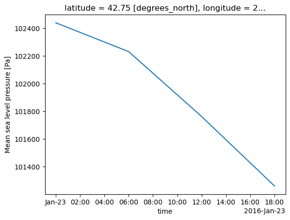
2. Dimension names
In Xarray, dimensions can be thought of as extensions of Pandas` 2-d row/column indices (aka axes). We can assign names, or labels, to Pandas indexes; in Xarray, these labeled axes are a necessary (and excellent) feature.
slp.dims('time', 'latitude', 'longitude')3. Coordinates
Coordinate variables in Xarray are 1-dimensional arrays that correspond to the Data variable’s dimensions.
In this case, slp has dimension coordinates of longitude, latitude, and time; each of these dimension coordinates consist of an array of values, plus metadata.
slp.coordsCoordinates:
* latitude (latitude) float32 3kB 90.0 89.75 89.5 ... -89.5 -89.75 -90.0
* longitude (longitude) float32 6kB 0.0 0.25 0.5 0.75 ... 359.2 359.5 359.8
* time (time) datetime64[ns] 32B 2016-01-23 ... 2016-01-23T18:00:00We can assign an object to each coordinate dimension.
lons = slp.longitudelats = slp.latitudetime = slp.timetime4. The data variables will typically have attributes (metadata) attached to them.
slp.attrs{'long_name': 'Mean sea level pressure',
'short_name': 'msl',
'standard_name': 'air_pressure_at_mean_sea_level',
'units': 'Pa'}slp.units'Pa'5. The coordinate variables will likely (but not always) have metadata as well.
lons.attrs{'long_name': 'longitude', 'units': 'degrees_east'}time.attrs{}Create a quick plan-view data visualization at a particular time.
slp.sel(time='2016-01-23-18:00:00').plot(figsize=(15,10))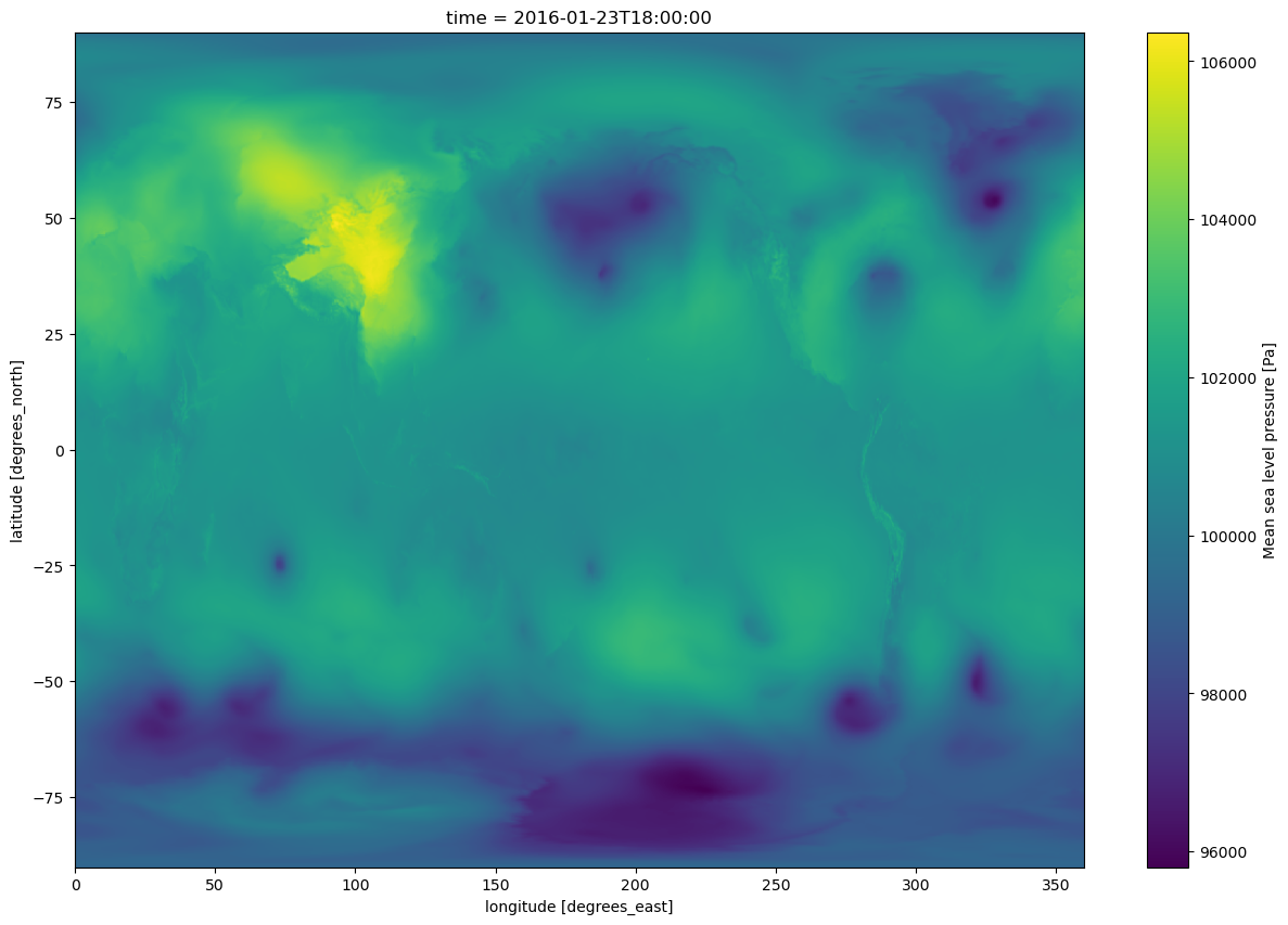
Explore this and other gridded datasets!
Now, try copying this notebook and make your own. Things to try in your own notebooks:
Read in a different variable (such as SST or any other variable of interest to you)
Create a time series and plan-view visualization of that variable
Read in, explore, and visualize data from the Global Ocean Physics Reanalysis. An example data file from this reanalysis is
/spare11/atm533/data/mercatorglorys12v1_gl12_mean_20250821_R20250827.nc.ADVANCED: Use MetPy to convert the units of a variable (e.g. from Kelvin to Celsius)
ADVANCED: Use Matplotlib and Cartopy and create a well-labeled line- or filled- contour plot over cartographic features
PRO: Overlay multiple variables on the same map
What's next?
We will learn more about data formats typically used to represent gridded data. We will also access datasets that are stored on remote servers.