Surface map of METAR data over a region#
Objective#
In this notebook, we will make a surface map based on current observations from worldwide METAR sites.
from datetime import datetime,timedelta
import numpy as np
import pandas as pd
import matplotlib.pyplot as plt

import cartopy.crs as ccrs
import cartopy.feature as cfeature

from metpy.calc import wind_components, reduce_point_density
from metpy.units import units
from metpy.plots import StationPlot, USCOUNTIES
from metpy.plots.wx_symbols import current_weather, sky_cover, wx_code_map

# Load in a collection of functions that process GEMPAK weather conditions and cloud cover data.
%run /kt11/ktyle/python/metargem.py
Determine the date and hour to gather observations #
# Use the current time, or set your own for a past time.
# Set current to False if you want to specify a past time.

nowTime = datetime.now()

current = True
#current = False
if (current):
    validTime = datetime.now()
    year = validTime.year
    month = validTime.month
    day = validTime.day
    hour = validTime.hour
    minute = validTime.minute
    validTime = datetime(year, month, day, hour, minute)
    offset = timedelta(minutes = 5)
    validTime = validTime - offset
else:
    year = 2010
    month = 2
    day = 5
    hour = 23
    minute = 0
    validTime = datetime(year, month, day, hour, minute)

timeStr = validTime.strftime("%Y-%m-%d %H UTC")
timeStr2 = validTime.strftime("%Y%m%d%H")
YYMMDDHH = validTime.strftime("%y%m%d%H")
print(timeStr)
print(validTime)
2025-04-03 18 UTC
2025-04-03 18:07:00
The METAR data are in hourly CSV files which can be opened by Pandas.#
metarFile = f'/ktyle_rit/scripts/sflist2/complete/{YYMMDDHH}.csv'
df = pd.read_csv(metarFile, sep='\\s+')
df
| STN | YYMMDD/HHMM | SLAT | SLON | SELV | PMSL | ALTI | TMPC | DWPC | SKNT | ... | P03C | CTYL | CTYM | CTYH | P06I | T6XC | T6NC | CEIL | P01I | SNEW | |
|---|---|---|---|---|---|---|---|---|---|---|---|---|---|---|---|---|---|---|---|---|---|
| 0 | DYS | 250403/1800 | 32.43 | -99.85 | 545.0 | 1009.7 | 29.85 | 13.1 | 7.3 | 12.0 | ... | 0.7 | -9999.0 | -9999.0 | -9999.0 | 0.0 | 13.1 | 10.7 | 21.0 | -9999.0 | -9999.0 |
| 1 | NUW | 250403/1800 | 48.35 | -122.65 | 14.0 | 1022.3 | 30.18 | 9.4 | 5.6 | 7.0 | ... | 1.4 | -9999.0 | -9999.0 | -9999.0 | -9999.0 | 9.4 | 4.4 | 35.0 | -9999.0 | -9999.0 |
| 2 | NYL | 250403/1800 | 32.65 | -114.62 | 65.0 | 1012.3 | 29.90 | 17.8 | 0.6 | 6.0 | ... | 0.9 | -9999.0 | -9999.0 | -9999.0 | -9999.0 | 17.8 | 10.6 | -9999.0 | -9999.0 | -9999.0 |
| 3 | PAIM | 250403/1800 | 66.00 | -153.70 | 389.0 | 1014.4 | 29.88 | -6.6 | -8.2 | 1.0 | ... | 0.3 | -9999.0 | -9999.0 | -9999.0 | -9999.0 | -6.4 | -11.1 | 25.0 | -9999.0 | -9999.0 |
| 4 | PAGA | 250403/1800 | 64.73 | -156.93 | 46.0 | 1015.6 | 29.98 | -6.7 | -9.4 | 4.0 | ... | 0.2 | -9999.0 | -9999.0 | -9999.0 | -9999.0 | -6.7 | -9.4 | -9999.0 | -9999.0 | -9999.0 |
| ... | ... | ... | ... | ... | ... | ... | ... | ... | ... | ... | ... | ... | ... | ... | ... | ... | ... | ... | ... | ... | ... |
| 4349 | LQBK | 250403/1800 | -9999.00 | -9999.00 | -9999.0 | -9999.0 | 30.12 | 13.0 | 8.0 | 3.0 | ... | -9999.0 | -9999.0 | -9999.0 | -9999.0 | -9999.0 | -9999.0 | -9999.0 | -9999.0 | -9999.0 | -9999.0 |
| 4350 | LQMO | 250403/1800 | -9999.00 | -9999.00 | -9999.0 | -9999.0 | 30.06 | 15.0 | 2.0 | 10.0 | ... | -9999.0 | -9999.0 | -9999.0 | -9999.0 | -9999.0 | -9999.0 | -9999.0 | -9999.0 | -9999.0 | -9999.0 |
| 4351 | LQTZ | 250403/1800 | -9999.00 | -9999.00 | -9999.0 | -9999.0 | 30.15 | 9.0 | 9.0 | 2.0 | ... | -9999.0 | -9999.0 | -9999.0 | -9999.0 | -9999.0 | -9999.0 | -9999.0 | 55.0 | -9999.0 | -9999.0 |
| 4352 | EGOP | 250403/1800 | -9999.00 | -9999.00 | -9999.0 | -9999.0 | 29.97 | 15.0 | 7.0 | 15.0 | ... | -9999.0 | -9999.0 | -9999.0 | -9999.0 | -9999.0 | -9999.0 | -9999.0 | 64.0 | -9999.0 | -9999.0 |
| 4353 | EGQA | 250403/1800 | -9999.00 | -9999.00 | -9999.0 | -9999.0 | 30.30 | 10.0 | 7.0 | 9.0 | ... | -9999.0 | -9999.0 | -9999.0 | -9999.0 | -9999.0 | -9999.0 | -9999.0 | -9999.0 | -9999.0 | -9999.0 |
4354 rows × 35 columns
Mapmaking made easy! Follow these steps:#
1. Set the bounds of your map.#
latN = 55
latS = 40
lonW = -78
lonE = -60

cLat = (latN + latS)/2
cLon = (lonW + lonE)/2
2. Select the projection (i.e. Cartopy’s coordinate reference system, aka CRS) for your map.#
proj_map = ccrs.LambertConformal(central_latitude=cLat, central_longitude=cLon)
3. Select the projection / CRS that is valid for the dataset you are plotting#
proj_data = ccrs.PlateCarree()
stationplotclass, we only need to perform this transformation once per Axes, when the class is first instantiated.4. Select the resolution of the Cartopy Natural Earth cartographic features.#
# Uncomment / comment as desired
res = '10m' # Most detailed, best for small regions (e.g. NYS)
#res = '50m' # Medium detail, best for medium-sized regions (e.g. CONUS)
#res = '110m' # Least detailed, best for large/global maps

res_county = '5m' # Use with MetPy's US County shapefiles
5. Select the cartographic features (e.g., physical ones such as coastlines or rivers, and political features like states or (national) borders) you will include in your maps.#
Dataset-specific customizations#
Perform the spatial subset.
df2 = df.query('SLAT >= @latS & SLAT <= @latN & SLON >= @lonW & SLON <= @lonE')
df2
| STN | YYMMDD/HHMM | SLAT | SLON | SELV | PMSL | ALTI | TMPC | DWPC | SKNT | ... | P03C | CTYL | CTYM | CTYH | P06I | T6XC | T6NC | CEIL | P01I | SNEW | |
|---|---|---|---|---|---|---|---|---|---|---|---|---|---|---|---|---|---|---|---|---|---|
| 8 | CACQ | 250403/1800 | 47.00 | -65.45 | 34.0 | 1021.8 | -9999.00 | -2.0 | -4.0 | 9.0 | ... | -9999.0 | -9999.0 | -9999.0 | -9999.0 | -9999.00 | -9999.0 | -9999.0 | -9999.0 | -9999.0 | -9999.0 |
| 9 | CAFC | 250403/1800 | 45.92 | -66.60 | 35.0 | 1019.2 | -9999.00 | -1.0 | -1.0 | 10.0 | ... | -9999.0 | -9999.0 | -9999.0 | -9999.0 | -9999.00 | -9999.0 | -9999.0 | -9999.0 | -9999.0 | -9999.0 |
| 10 | CAFY | 250403/1800 | 45.60 | -64.95 | 43.0 | -9999.0 | -9999.00 | -1.0 | -2.0 | 2.0 | ... | -9999.0 | -9999.0 | -9999.0 | -9999.0 | -9999.00 | -9999.0 | -9999.0 | -9999.0 | -9999.0 | -9999.0 |
| 11 | CAKC | 250403/1800 | 46.77 | -65.00 | 34.0 | 1022.5 | -9999.00 | -2.0 | -4.0 | 5.0 | ... | -9999.0 | -9999.0 | -9999.0 | -9999.0 | -9999.00 | -9999.0 | -9999.0 | -9999.0 | -9999.0 | -9999.0 |
| 12 | CAOH | 250403/1800 | 45.23 | -63.05 | 24.0 | 1025.9 | -9999.00 | -1.0 | -2.0 | 7.0 | ... | -9999.0 | -9999.0 | -9999.0 | -9999.0 | -9999.00 | -9999.0 | -9999.0 | -9999.0 | -9999.0 | -9999.0 |
| ... | ... | ... | ... | ... | ... | ... | ... | ... | ... | ... | ... | ... | ... | ... | ... | ... | ... | ... | ... | ... | ... |
| 3704 | 6B0 | 250403/1800 | 43.99 | -73.10 | 149.0 | -9999.0 | 29.84 | 12.2 | 10.8 | 10.0 | ... | -9999.0 | -9999.0 | -9999.0 | -9999.0 | 0.06 | 12.2 | 4.1 | 20.0 | -9999.0 | -9999.0 |
| 3878 | XLL | 250403/1800 | 40.57 | -75.49 | 122.0 | -9999.0 | 30.04 | 19.0 | 15.0 | 7.0 | ... | -9999.0 | -9999.0 | -9999.0 | -9999.0 | -9999.00 | -9999.0 | -9999.0 | -9999.0 | -9999.0 | -9999.0 |
| 3896 | ZER | 250403/1800 | 40.71 | -76.37 | 527.0 | -9999.0 | 30.03 | 18.0 | 13.0 | 11.0 | ... | -9999.0 | -9999.0 | -9999.0 | -9999.0 | -9999.00 | -9999.0 | -9999.0 | -9999.0 | -9999.0 | -9999.0 |
| 4060 | 4B8 | 250403/1800 | 41.69 | -72.86 | 61.0 | -9999.0 | 29.99 | 12.9 | 12.9 | 6.0 | ... | -9999.0 | -9999.0 | -9999.0 | -9999.0 | -9999.00 | -9999.0 | -9999.0 | 7.0 | -9999.0 | -9999.0 |
| 4095 | JPX | 250403/1800 | 40.95 | -72.25 | 10.0 | -9999.0 | 30.04 | 11.0 | 11.0 | 12.0 | ... | -9999.0 | -9999.0 | -9999.0 | -9999.0 | 0.60 | 11.0 | 7.7 | 2.0 | -9999.0 | -9999.0 |
275 rows × 35 columns
Select the weather variables of interest. Also include the site ID, lat, lon, elevation, and time columns.
columnSubset = ['STN', 'YYMMDD/HHMM', 'SLAT', 'SLON', 'SELV', 'TMPC', 'DWPC', 'PMSL',
                'SKNT', 'DRCT','ALTI','WNUM','VSBY','CHC1', 'CHC2', 'CHC3','CTYH', 'CTYM', 'CTYL']
df3 = df2[columnSubset]
df3
| STN | YYMMDD/HHMM | SLAT | SLON | SELV | TMPC | DWPC | PMSL | SKNT | DRCT | ALTI | WNUM | VSBY | CHC1 | CHC2 | CHC3 | CTYH | CTYM | CTYL | |
|---|---|---|---|---|---|---|---|---|---|---|---|---|---|---|---|---|---|---|---|
| 8 | CACQ | 250403/1800 | 47.00 | -65.45 | 34.0 | -2.0 | -4.0 | 1021.8 | 9.0 | 110.0 | -9999.00 | -9999.0 | -9999.0 | -9999.0 | -9999.0 | -9999.0 | -9999.0 | -9999.0 | -9999.0 |
| 9 | CAFC | 250403/1800 | 45.92 | -66.60 | 35.0 | -1.0 | -1.0 | 1019.2 | 10.0 | 110.0 | -9999.00 | -9999.0 | -9999.0 | -9999.0 | -9999.0 | -9999.0 | -9999.0 | -9999.0 | -9999.0 |
| 10 | CAFY | 250403/1800 | 45.60 | -64.95 | 43.0 | -1.0 | -2.0 | -9999.0 | 2.0 | 190.0 | -9999.00 | -9999.0 | -9999.0 | -9999.0 | -9999.0 | -9999.0 | -9999.0 | -9999.0 | -9999.0 |
| 11 | CAKC | 250403/1800 | 46.77 | -65.00 | 34.0 | -2.0 | -4.0 | 1022.5 | 5.0 | 140.0 | -9999.00 | -9999.0 | -9999.0 | -9999.0 | -9999.0 | -9999.0 | -9999.0 | -9999.0 | -9999.0 |
| 12 | CAOH | 250403/1800 | 45.23 | -63.05 | 24.0 | -1.0 | -2.0 | 1025.9 | 7.0 | 150.0 | -9999.00 | -9999.0 | -9999.0 | -9999.0 | -9999.0 | -9999.0 | -9999.0 | -9999.0 | -9999.0 |
| ... | ... | ... | ... | ... | ... | ... | ... | ... | ... | ... | ... | ... | ... | ... | ... | ... | ... | ... | ... |
| 3704 | 6B0 | 250403/1800 | 43.99 | -73.10 | 149.0 | 12.2 | 10.8 | -9999.0 | 10.0 | 180.0 | 29.84 | -9999.0 | 10.0 | 204.0 | -9999.0 | -9999.0 | -9999.0 | -9999.0 | -9999.0 |
| 3878 | XLL | 250403/1800 | 40.57 | -75.49 | 122.0 | 19.0 | 15.0 | -9999.0 | 7.0 | 240.0 | 30.04 | -9999.0 | 10.0 | 1.0 | -9999.0 | -9999.0 | -9999.0 | -9999.0 | -9999.0 |
| 3896 | ZER | 250403/1800 | 40.71 | -76.37 | 527.0 | 18.0 | 13.0 | -9999.0 | 11.0 | 220.0 | 30.03 | -9999.0 | 10.0 | 1.0 | -9999.0 | -9999.0 | -9999.0 | -9999.0 | -9999.0 |
| 4060 | 4B8 | 250403/1800 | 41.69 | -72.86 | 61.0 | 12.9 | 12.9 | -9999.0 | 6.0 | 150.0 | 29.99 | 9.0 | 6.0 | 74.0 | -9999.0 | -9999.0 | -9999.0 | -9999.0 | -9999.0 |
| 4095 | JPX | 250403/1800 | 40.95 | -72.25 | 10.0 | 11.0 | 11.0 | -9999.0 | 12.0 | 230.0 | 30.04 | 9.0 | 0.5 | 24.0 | -9999.0 | -9999.0 | -9999.0 | -9999.0 | -9999.0 |
275 rows × 19 columns
In these datasets, -9999.0 signfies missing values. Replace all instances of -9999.0 with NumPy’s NaN (not a number) value.
df4 = df3.replace(-9999.0, np.nan)
df4
| STN | YYMMDD/HHMM | SLAT | SLON | SELV | TMPC | DWPC | PMSL | SKNT | DRCT | ALTI | WNUM | VSBY | CHC1 | CHC2 | CHC3 | CTYH | CTYM | CTYL | |
|---|---|---|---|---|---|---|---|---|---|---|---|---|---|---|---|---|---|---|---|
| 8 | CACQ | 250403/1800 | 47.00 | -65.45 | 34.0 | -2.0 | -4.0 | 1021.8 | 9.0 | 110.0 | NaN | NaN | NaN | NaN | NaN | NaN | NaN | NaN | NaN |
| 9 | CAFC | 250403/1800 | 45.92 | -66.60 | 35.0 | -1.0 | -1.0 | 1019.2 | 10.0 | 110.0 | NaN | NaN | NaN | NaN | NaN | NaN | NaN | NaN | NaN |
| 10 | CAFY | 250403/1800 | 45.60 | -64.95 | 43.0 | -1.0 | -2.0 | NaN | 2.0 | 190.0 | NaN | NaN | NaN | NaN | NaN | NaN | NaN | NaN | NaN |
| 11 | CAKC | 250403/1800 | 46.77 | -65.00 | 34.0 | -2.0 | -4.0 | 1022.5 | 5.0 | 140.0 | NaN | NaN | NaN | NaN | NaN | NaN | NaN | NaN | NaN |
| 12 | CAOH | 250403/1800 | 45.23 | -63.05 | 24.0 | -1.0 | -2.0 | 1025.9 | 7.0 | 150.0 | NaN | NaN | NaN | NaN | NaN | NaN | NaN | NaN | NaN |
| ... | ... | ... | ... | ... | ... | ... | ... | ... | ... | ... | ... | ... | ... | ... | ... | ... | ... | ... | ... |
| 3704 | 6B0 | 250403/1800 | 43.99 | -73.10 | 149.0 | 12.2 | 10.8 | NaN | 10.0 | 180.0 | 29.84 | NaN | 10.0 | 204.0 | NaN | NaN | NaN | NaN | NaN |
| 3878 | XLL | 250403/1800 | 40.57 | -75.49 | 122.0 | 19.0 | 15.0 | NaN | 7.0 | 240.0 | 30.04 | NaN | 10.0 | 1.0 | NaN | NaN | NaN | NaN | NaN |
| 3896 | ZER | 250403/1800 | 40.71 | -76.37 | 527.0 | 18.0 | 13.0 | NaN | 11.0 | 220.0 | 30.03 | NaN | 10.0 | 1.0 | NaN | NaN | NaN | NaN | NaN |
| 4060 | 4B8 | 250403/1800 | 41.69 | -72.86 | 61.0 | 12.9 | 12.9 | NaN | 6.0 | 150.0 | 29.99 | 9.0 | 6.0 | 74.0 | NaN | NaN | NaN | NaN | NaN |
| 4095 | JPX | 250403/1800 | 40.95 | -72.25 | 10.0 | 11.0 | 11.0 | NaN | 12.0 | 230.0 | 30.04 | 9.0 | 0.5 | 24.0 | NaN | NaN | NaN | NaN | NaN |
275 rows × 19 columns
Now that we have done our subsetting, create a generic object (we’ll call it data here)
data = df4
In our current data archive, multiple weather types are often not represented properly. To avoid a type conversion error, set stations whose weather type fall into this category to missing.
This will eventually be fixed!
data.loc[data['WNUM'] =='********', ['WNUM']] = '-9999.00'
data['WNUM'] = data['WNUM'].astype('float16')
/tmp/ipykernel_3403159/3580734062.py:1: FutureWarning: Setting an item of incompatible dtype is deprecated and will raise an error in a future version of pandas. Value '-9999.00' has dtype incompatible with float64, please explicitly cast to a compatible dtype first.
  data.loc[data['WNUM'] =='********', ['WNUM']] = '-9999.00'
Read in several of the columns as Pandas Series; extract the value arrays from the Series objects; assign / convert units as necessary; convert GEMPAK cloud cover and present wx symbols to MetPy’s representation#
lats = data['SLAT'].values
lons = data['SLON'].values
tair = (data['TMPC'].values * units ('degC')).to('degF')
dewp = (data['DWPC'].values * units ('degC')).to('degF')
altm = (data['ALTI'].values * units('inHg')).to('mbar')
slp = data['PMSL'].values * units('hPa')

# Convert wind to components
u, v = wind_components(data['SKNT'].values * units.knots, data['DRCT'].values * units.degree)

# replace missing wx codes or those >= 100 with 0, and convert to MetPy's present weather code
wnum = (np.nan_to_num(data['WNUM'].values,True).astype(int))
convert_wnum (wnum)

# Need to handle missing (NaN) and convert to proper code
chc1 = (np.nan_to_num(data['CHC1'].values,True).astype(int))
chc2 = (np.nan_to_num(data['CHC2'].values,True).astype(int))
chc3 = (np.nan_to_num(data['CHC3'].values,True).astype(int))
cloud_cover = calc_clouds(chc1, chc2, chc3)

# Set a variable to be used for plotting the station ID's
stid = data['STN']
The next step deals with the removal of overlapping stations, using reduce_point_density. This returns a mask we can apply to data to filter the points.
density to an appropriate spacing (in meters) for the region you selected. Play around with it until you reach an ideal blend of coverage and readability.# Project points so that we're filtering based on the way the stations are represented in the dataset
xy = proj_map.transform_points(proj_data, lons, lats)
# Reduce point density so that there's only one point within a circle whose distance is specified in meters.
# This value will need to change depending on how large of an area you are plotting.
density = 40000
mask = reduce_point_density(xy, density)
transform_points, we pass in the arrays of the stations' longitudes and latitudes. Since their units are in degrees, we need to also specify their corresponding map projection (PlateCarree) ... which we defined earlier in Mapmaking Made Easy Step 2.Simple station plotting using plot methods#
One way to create station plots with MetPy is to create an instance of StationPlot and call various plot methods, like plot_parameter, to plot arrays of data at locations relative to the center point.
In addition to plotting values, StationPlot has support for plotting text strings, symbols, and plotting values using custom formatting.
Plotting symbols involves mapping integer values to various custom font glyphs in our custom weather symbols font. MetPy provides mappings for converting WMO codes to their appropriate symbol. The sky_cover and current_weather functions below are two such mappings.
Now we just plot with arr[mask] for every arr of data we use in plotting.
- Play with the values of dpi and figsize, and see how changes affect the look of your map.
- Adjust the the bounds of the longitudinal/latitudinal extents (w_ext, e_ext, s_ext, n_ext) until you maximize coverage near the bounds of your map, without having any text appearing outside the frame. You'll need to pay attention to the signs of these values (see the previous in-class examples)!
- Experiment with different cartographic features, and/or change their attributes (e.g., thickness, linetype, color, etc.)
- Experiment with different font sizes and colors for the
stationplotbase class itself and/or its individual parameters.
# Set up a plot with map features
# First set dpi ("dots per inch") - higher values will give us a less pixelated final figure. Default is 100.
dpi = 125
# Set figure size. Default is 11x8.5
fig = plt.figure(figsize=(30, 24), dpi=dpi)
# Mapmaking Made Easy Step 2
ax = fig.add_subplot(1, 1, 1, projection=proj_map)
# Mapmaking Made Easy Step 1
# Slightly expand the extent of the map as compared to the subsetted data region; this helps eliminate data from being plotted beyond the frame of the map
w_ext = -0.2
e_ext = 0.2
s_ext = -0.2
n_ext = 0.2
ax.set_extent ((lonW + w_ext,lonE + e_ext,latS + s_ext, latN + n_ext), crs=proj_data)
# Mapmaking Made Easy Step 5
ax.set_facecolor(cfeature.COLORS['water'])
land_mask = cfeature.NaturalEarthFeature('physical', 'land', res,
edgecolor='face',
facecolor=cfeature.COLORS['land'])
lake_mask = cfeature.NaturalEarthFeature('physical', 'lakes', res,
edgecolor='face',
facecolor=cfeature.COLORS['water'])
state_borders = cfeature.NaturalEarthFeature(category='cultural', name='admin_1_states_provinces_lakes',
scale=res, facecolor='none')
ax.add_feature(land_mask)
ax.add_feature(lake_mask)
ax.add_feature(state_borders, linestyle='solid', edgecolor='black')
#If we wanted to add grid lines to our plot:
#ax.gridlines()
# Create a station plot pointing to an Axes to draw on as well as the location of points
stationplot = StationPlot(ax, lons[mask], lats[mask], transform=proj_data,
fontsize=8)
stationplot.plot_parameter('NW', tair[mask], color='red', fontsize=10)
stationplot.plot_parameter('SW', dewp[mask], color='darkgreen', fontsize=10)
# Below, we are using a custom formatter to control how the sea-level pressure
# values are plotted. This uses the standard trailing 3-digits of the pressure value
# in tenths of millibars.
stationplot.plot_parameter('NE', slp[mask], color='purple', formatter=lambda v: format(10 * v, '.0f')[-3:])
stationplot.plot_symbol('C', cloud_cover[mask], sky_cover)
stationplot.plot_symbol('W', wnum[mask], current_weather,color='blue',fontsize=12)
stationplot.plot_text((2, 0),stid[mask], color='gray')
#zorder - Higher value zorder will plot the variable on top of lower value zorder. This is necessary for wind barbs to appear. Default is 1.
stationplot.plot_barb(u[mask], v[mask],zorder=2)
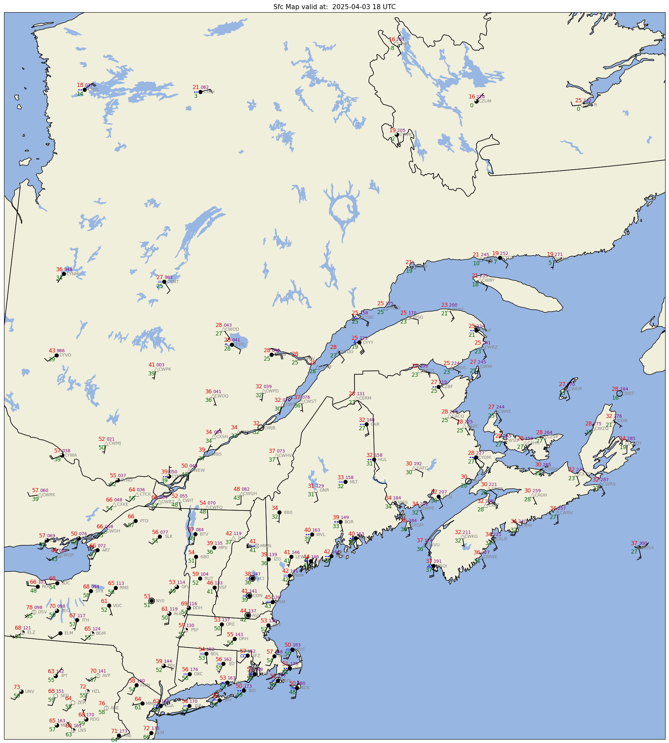
plotTitle = (f"Sfc Map valid at: {timeStr}")
ax.set_title (plotTitle);
# In order to see the entire figure, type the name of the figure object below.
fig
Save the figure as a PNG.#
- Set a variable to a string that represents your map region. Use that variable in the
fig_name.
region = 'Atlantic_Canada'
figName = (f'{timeStr2}_{region}_sfmap.png')
fig.savefig(figName)
- Re-run the notebook; try a different region and/or select a past date (within the last couple years) and time.