02_GriddedDiagnostics_Dewpoint_ERA5#
In this notebook, we’ll cover the following:#
Select a date and access an ERA5 Dataset
Subset the desired Datasets along their dimensions
Calculate and visualize dewpoint.
0) Imports #
import xarray as xr
import pandas as pd
import numpy as np
from datetime import datetime as dt
from metpy.units import units
import metpy.calc as mpcalc
import cartopy.crs as ccrs
import cartopy.feature as cfeature
import matplotlib.pyplot as plt
1) Specify a starting and ending date/time, regional extent, vertical levels, and access the ERA5#
# Areal extent
lonW = -105
lonE = -90
latS = 31
latN = 39
cLat, cLon = (latS + latN)/2, (lonW + lonE)/2

# Recall that in ERA5, longitudes run between 0 and 360, not -180 and 180
if (lonW < 0 ):
    lonW = lonW + 360
if (lonE < 0 ):
    lonE = lonE + 360

expand = 1
latRange = np.arange(latS - expand,latN + expand,.25) # expand the data range a bit beyond the plot range
lonRange = np.arange((lonW - expand),(lonE + expand),.25) # Need to match longitude values to those of the coordinate variable

# Vertical level specification
pLevel = 925
levStr = f'{pLevel}'

startYear = 2013
startMonth = 5
startDay = 31
startHour = 12
startMinute = 0
startDateTime = dt(startYear,startMonth,startDay, startHour, startMinute)

endYear = 2013
endMonth = 5
endDay = 31
endHour = 18
endMinute = 0
endDateTime = dt(endYear,endMonth,endDay, endHour, endMinute)

delta_time = endDateTime - startDateTime
time_range_max = 7*86400

if (delta_time.total_seconds() > time_range_max):
        raise RuntimeError("Your time range must not exceed 7 days. Go back and try again.")
Wb2EndDate = dt(2023,1,10)
if (endDateTime <= Wb2EndDate):
    ds = xr.open_dataset(
     'gs://weatherbench2/datasets/era5/1959-2023_01_10-wb13-6h-1440x721.zarr',
     chunks={'time': 48},
     consolidated=True,
     engine='zarr'
)
else:
    import glob, os
    input_directory = '/free/ktyle/era5'
    files = glob.glob(os.path.join(input_directory,'*.nc'))
    varDict = {'valid_time': 'time',
               'pressure_level': 'level',
               'msl': 'mean_sea_level_pressure',
               'q': 'specific_humidity',
               't': 'temperature',
               'u': 'u_component_of_wind',
               'v': 'v_component_of_wind',
               'w': 'vertical_velocity',
               'z': 'geopotential'}
    dimDict = {'valid_time': 'time',
               'pressure_level': 'level'}
    ds = xr.open_mfdataset(files).rename_dims(dimDict).rename_vars(varDict)
Examine the Dataset
ds
<xarray.Dataset> Size: 47TB
Dimensions:                                           (time: 93544,
                                                       latitude: 721,
                                                       longitude: 1440,
                                                       level: 13)
Coordinates:
  * latitude                                          (latitude) float32 3kB ...
  * level                                             (level) int64 104B 50 ....
  * longitude                                         (longitude) float32 6kB ...
  * time                                              (time) datetime64[ns] 748kB ...
Data variables: (12/50)
    10m_u_component_of_wind                           (time, latitude, longitude) float32 388GB dask.array<chunksize=(48, 721, 1440), meta=np.ndarray>
    10m_v_component_of_wind                           (time, latitude, longitude) float32 388GB dask.array<chunksize=(48, 721, 1440), meta=np.ndarray>
    2m_dewpoint_temperature                           (time, latitude, longitude) float32 388GB dask.array<chunksize=(48, 721, 1440), meta=np.ndarray>
    2m_temperature                                    (time, latitude, longitude) float32 388GB dask.array<chunksize=(48, 721, 1440), meta=np.ndarray>
    angle_of_sub_gridscale_orography                  (latitude, longitude) float32 4MB dask.array<chunksize=(721, 1440), meta=np.ndarray>
    anisotropy_of_sub_gridscale_orography             (latitude, longitude) float32 4MB dask.array<chunksize=(721, 1440), meta=np.ndarray>
    ...                                                ...
    v_component_of_wind                               (time, level, latitude, longitude) float32 5TB dask.array<chunksize=(48, 13, 721, 1440), meta=np.ndarray>
    vertical_velocity                                 (time, level, latitude, longitude) float32 5TB dask.array<chunksize=(48, 13, 721, 1440), meta=np.ndarray>
    volumetric_soil_water_layer_1                     (time, latitude, longitude) float32 388GB dask.array<chunksize=(48, 721, 1440), meta=np.ndarray>
    volumetric_soil_water_layer_2                     (time, latitude, longitude) float32 388GB dask.array<chunksize=(48, 721, 1440), meta=np.ndarray>
    volumetric_soil_water_layer_3                     (time, latitude, longitude) float32 388GB dask.array<chunksize=(48, 721, 1440), meta=np.ndarray>
volumetric_soil_water_layer_4 (time, latitude, longitude) float32 388GB dask.array<chunksize=(48, 721, 1440), meta=np.ndarray>2) Specify a date/time range, and subset the desired Datasets along their dimensions.#
Create a list of date and times based on what we specified for the initial and final times, using Pandas’ date_range function
dateList = pd.date_range(startDateTime, endDateTime,freq="6h")
dateList
DatetimeIndex(['2013-05-31 12:00:00', '2013-05-31 18:00:00'], dtype='datetime64[ns]', freq='6h')
We will calculate dewpoint, which depends on temperature and specific humidity (and also pressure, as we will see), so read in those arrays. Read in U and V as well if we wish to visualize wind vectors.
Now create objects for our desired DataArrays based on the coordinates we have subsetted.#
# Data variable selection
Q = ds['specific_humidity'].sel(time=dateList,level=pLevel,latitude=latRange,longitude=lonRange).compute()
T = ds['temperature'].sel(time=dateList,level=pLevel,latitude=latRange,longitude=lonRange).compute()
U = ds['u_component_of_wind'].sel(time=dateList,level=pLevel,latitude=latRange,longitude=lonRange).compute()
V = ds['v_component_of_wind'].sel(time=dateList,level=pLevel,latitude=latRange,longitude=lonRange).compute()
Define our subsetted coordinate arrays of lat and lon. Pull them from any of the DataArrays. We’ll need to pass these into the contouring functions later on.
lats = T.latitude
lons = T.longitude
3) Calculate and visualize dewpoint.#
Let’s examine the MetPy diagnostic that calculates dewpoint if specific humidity is available: Dewpoint from specific humidity
We can see that this function requires us to pass in arrays of pressure, temperature, and specific humidity. In this case, pressure is constant everywhere, since we are operating on an isobaric surface.
As such, we need to be sure we are attaching units to our previously specified pressure level.
#Attach units to pLevel for use in MetPy with new variable, P:
P = pLevel*units['hPa']
P
Now, we have everything we need to calculate dewpoint.
Td = mpcalc.dewpoint_from_specific_humidity(P, T, Q)
Td
<xarray.DataArray (time: 2, latitude: 40, longitude: 68)> Size: 22kB
<Quantity([[[ -1.4107361  -1.5895691  -2.0344543 ...  16.597534   16.575531
    16.493134 ]
  [ -1.367218   -1.5028381  -1.9390869 ...  16.802917   16.93866
    16.890442 ]
  [ -1.323822   -1.4874573  -1.8988953 ...  17.151154   17.256256
    17.26233  ]
  ...
  [ -4.227661   -5.0594788  -6.6793213 ...  15.957611   16.10202
    16.119781 ]
  [ -4.5113525  -6.3446655  -6.4185486 ...  16.090698   16.256866
    16.36029  ]
  [ -5.3642883  -5.3642883  -5.316864  ...  15.911102   16.079376
    16.236053 ]]

 [[  1.7564392   1.5214844   0.9430237 ...  16.297668   16.021454
    16.296082 ]
  [  2.5342712   1.8949585   1.297821  ...  17.01474    16.60028
    16.73642  ]
  [  2.7510376   2.0981445   1.5380554 ...  18.092377   18.070343
    17.842682 ]
  ...
  [-11.552734  -12.473419  -13.109833  ...  15.016998   14.938568
    15.207672 ]
  [-12.275909  -12.900482  -13.152069  ...  15.116882   14.95282
    14.871918 ]
  [-11.095917  -11.395691  -10.156097  ...  15.289978   15.064209
    14.78064  ]]], 'degree_Celsius')>
Coordinates:
  * latitude   (latitude) float32 160B 30.0 30.25 30.5 ... 39.25 39.5 39.75
    level      int64 8B 925
  * longitude  (longitude) float32 272B 254.0 254.2 254.5 ... 270.2 270.5 270.8
* time (time) datetime64[ns] 16B 2013-05-31T12:00:00 2013-05-31T18:00:00Notice the units are in degrees Celsius.
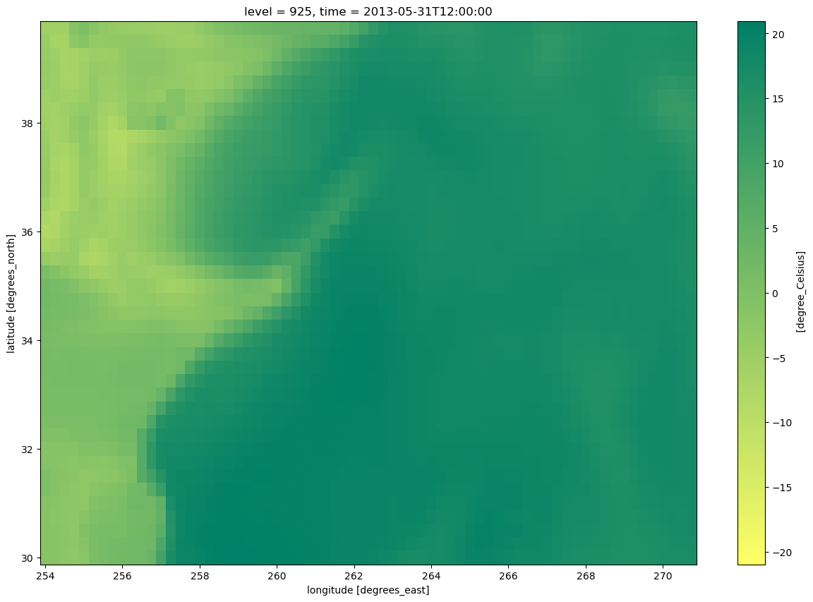
Let’s do a quick visualization.
Td.sel(time=startDateTime).plot(figsize=(15,10),cmap='summer_r')
<matplotlib.collections.QuadMesh at 0x151f6b8ac320>
Find the min/max values (no scaling necessary). Use these to inform the setting of the contour fill intervals.#
minTd = Td.min().values
maxTd = Td.max().values
print (minTd, maxTd)
-13.152069 20.966217
TdInc = 2
TdContours = np.arange (-12, 24, TdInc)
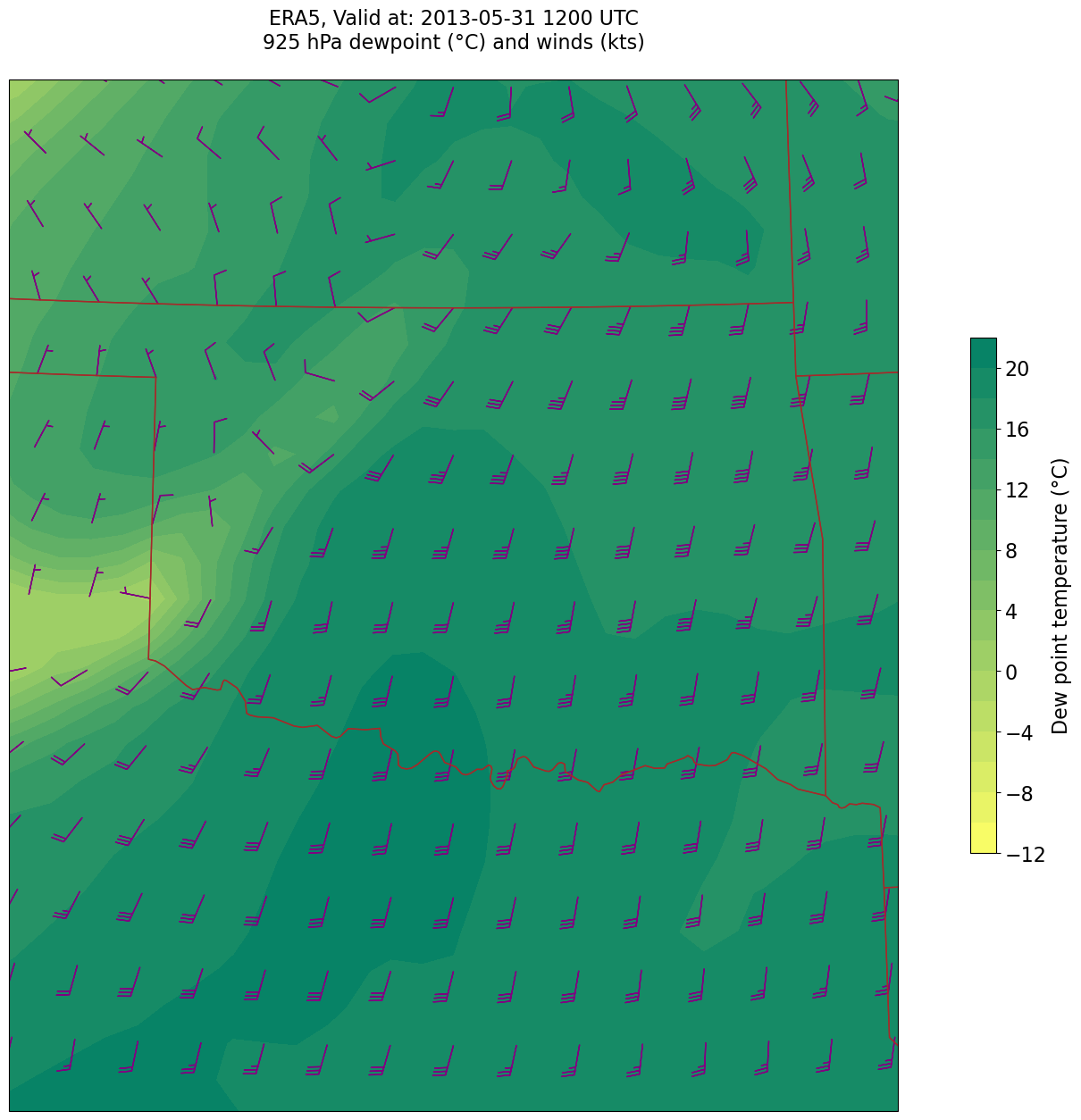
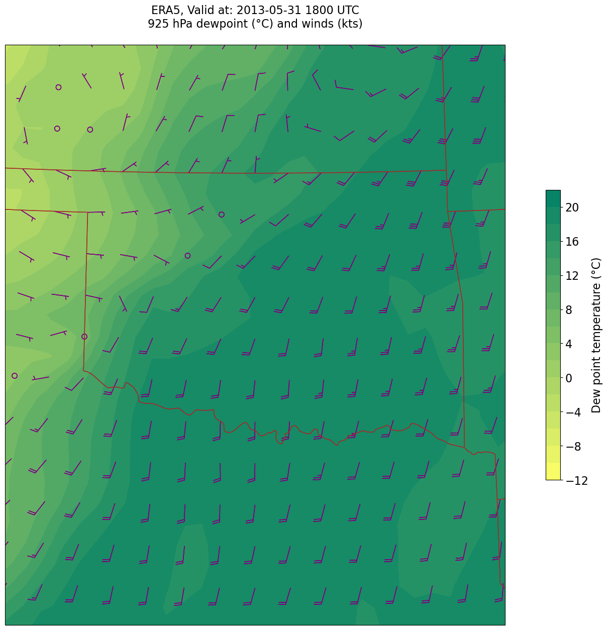
Now, let’s plot filled contours of dewpoint, and wind barbs on the map.#
Convert U and V to knots
UKts = U.metpy.convert_units('kts')
VKts = V.metpy.convert_units('kts')
constrainLat, constrainLon = (0.5, 4.0)
proj_map = ccrs.LambertConformal(central_longitude=cLon, central_latitude=cLat)
proj_data = ccrs.PlateCarree() # Our data is lat-lon; thus its native projection is Plate Carree.
res = '50m'
for time in dateList:
    print("Processing", time)

    # Create the time strings, for the figure title as well as for the file name.
    timeStr = dt.strftime(time,format="%Y-%m-%d %H%M UTC")
    timeStrFile = dt.strftime(time,format="%Y%m%d%H")

    tl1 = f'ERA5, Valid at: {timeStr}'
    tl2 = f'{levStr} hPa dewpoint (°C) and winds (kts)'

    title_line = f'{tl1}\n{tl2}\n'

    fig = plt.figure(figsize=(21,15)) # Increase size to adjust for the constrained lats/lons
    ax = fig.add_subplot(1,1,1,projection=proj_map)
    ax.set_extent ([lonW+constrainLon,lonE-constrainLon,latS+constrainLat,latN-constrainLat])
    ax.add_feature(cfeature.COASTLINE.with_scale(res))
    ax.add_feature(cfeature.STATES.with_scale(res),edgecolor='brown')

    # Need to use Xarray's sel method here to specify the current time for any DataArray you are plotting.

    # 1. Contour fill of dewpoint.
    cTd = ax.contourf(lons, lats, Td.sel(time=time), levels=TdContours, cmap='summer_r', transform=proj_data)
    cbar = plt.colorbar(cTd,shrink=0.5)
    cbar.ax.tick_params(labelsize=16)
    cbar.ax.set_ylabel("Dew point temperature (°C)",fontsize=16)

    # 4. wind barbs
    # Plotting wind barbs uses the ax.barbs method. Here, you can't pass in the DataArray directly; you can only pass in the array's values.
    # Also need to sample (skip) a selected # of points to keep the plot readable.
    # Remember to use Xarray's sel method here as well to specify the current time.
    skip = 2
    ax.barbs(lons[::skip],lats[::skip],UKts.sel(time=time)[::skip,::skip].values, VKts.sel(time=time)[::skip,::skip].values, color='purple',transform=proj_data)

    title = ax.set_title(title_line,fontsize=16)
    #Generate a string for the file name and save the graphic to your current directory.
    fileName = f'{timeStrFile}_ERA5_{levStr}_Td_Wind.png'
    fig.savefig(fileName)
Processing 2013-05-31 12:00:00
Processing 2013-05-31 18:00:00