03_Xarray: Overlays of variables#
Overview#
Work with multiple Xarray
DatasetsSubset the Dataset along its dimensions
Perform unit conversions
Create a well-labeled multi-parameter contour plot of gridded ERA5 data
Imports#
import xarray as xr
import pandas as pd
import numpy as np
from datetime import datetime as dt
from metpy.units import units
import metpy.calc as mpcalc
import cartopy.crs as ccrs
import cartopy.feature as cfeature
import matplotlib.pyplot as plt
Work with an Xarray Dataset#
ds = xr.open_dataset('/spare11/atm350/data/199303_era5.nc')
Examine the dataset
ds
<xarray.Dataset> Size: 7GB
Dimensions:                  (latitude: 721, level: 13, longitude: 1440,
                              time: 124)
Coordinates:
  * latitude                 (latitude) float32 3kB 90.0 89.75 ... -89.75 -90.0
  * level                    (level) int64 104B 50 100 150 200 ... 850 925 1000
  * longitude                (longitude) float32 6kB 0.0 0.25 ... 359.5 359.8
  * time                     (time) datetime64[ns] 992B 1993-03-01 ... 1993-0...
Data variables:
    geopotential             (time, level, latitude, longitude) float32 7GB ...
mean_sea_level_pressure (time, latitude, longitude) float32 515MB ...Subset the Datasets along their dimensions#
We noticed in the previous notebook that our contour labels were not appearing with every contour line. This is because we passed the entire horizontal extent (all latitudes and longitudes) to the ax.contour method. Since our intent is to plot only over a regional subset, we will use the sel method on the latitude and longitude dimensions as well as time and isobaric surface.
We’ll retrieve two data variables, geopotential and sea-level pressure, from the Dataset.
We’ll also use Datetime and string methods to more dynamically assign various dimensional specifications, as well as aid in figure-labeling later on.
# Areal extent

lonW = -100
lonE = -60
latS = 25
latN = 55
cLat, cLon = (latS + latN)/2, (lonW + lonE)/2

# Recall that in ERA5, longitudes run between 0 and 360, not -180 and 180
if (lonW < 0 ):
    lonW = lonW + 360
if (lonE < 0 ):
    lonE = lonE + 360

expand = 1
latRange = np.arange(latS - expand,latN + expand,.5) # expand the data range a bit beyond the plot range
lonRange = np.arange((lonW - expand),(lonE + expand),.5) # Need to match longitude values to those of the coordinate variable

# Vertical level specificaton
plevel = 500
levelStr = str(plevel)

# Date/Time specification
Year = 1993
Month = 3
Day = 14
Hour = 12
Minute = 0
dateTime = dt(Year,Month,Day, Hour, Minute)
timeStr = dateTime.strftime("%Y-%m-%d %H%M UTC")

# Data variable selection

z = ds['geopotential'].sel(time=dateTime,level=plevel,latitude=latRange,longitude=lonRange)
slp = ds['mean_sea_level_pressure'].sel(time=dateTime,latitude=latRange,longitude=lonRange) # of course, no isobaric surface for SLP
levelStr
'500'
timeStr
'1993-03-14 1200 UTC'
Let’s look at some of the attributes
z.shape
(64, 84)
z.dims
('latitude', 'longitude')
As a result of selecting just a single time and isobaric surface, both of those dimensions have been abstracted out of the DataArray.
z.units
'm**2 s**-2'
slp.shape
(64, 84)
slp.dims
('latitude', 'longitude')
slp.units
'Pa'
Define our subsetted coordinate arrays of lat and lon. Pull them from either of the two DataArrays. We’ll need to pass these into the contouring functions later on.#
lats = z.latitude
lons = z.longitude
lats
<xarray.DataArray 'latitude' (latitude: 64)> Size: 256B
array([24. , 24.5, 25. , 25.5, 26. , 26.5, 27. , 27.5, 28. , 28.5, 29. , 29.5,
       30. , 30.5, 31. , 31.5, 32. , 32.5, 33. , 33.5, 34. , 34.5, 35. , 35.5,
       36. , 36.5, 37. , 37.5, 38. , 38.5, 39. , 39.5, 40. , 40.5, 41. , 41.5,
       42. , 42.5, 43. , 43.5, 44. , 44.5, 45. , 45.5, 46. , 46.5, 47. , 47.5,
       48. , 48.5, 49. , 49.5, 50. , 50.5, 51. , 51.5, 52. , 52.5, 53. , 53.5,
       54. , 54.5, 55. , 55.5], dtype=float32)
Coordinates:
  * latitude  (latitude) float32 256B 24.0 24.5 25.0 25.5 ... 54.5 55.0 55.5
    level     int64 8B 500
    time      datetime64[ns] 8B 1993-03-14T12:00:00
Attributes:
    long_name:  latitude
units: degrees_northlons
<xarray.DataArray 'longitude' (longitude: 84)> Size: 336B
array([259. , 259.5, 260. , 260.5, 261. , 261.5, 262. , 262.5, 263. , 263.5,
       264. , 264.5, 265. , 265.5, 266. , 266.5, 267. , 267.5, 268. , 268.5,
       269. , 269.5, 270. , 270.5, 271. , 271.5, 272. , 272.5, 273. , 273.5,
       274. , 274.5, 275. , 275.5, 276. , 276.5, 277. , 277.5, 278. , 278.5,
       279. , 279.5, 280. , 280.5, 281. , 281.5, 282. , 282.5, 283. , 283.5,
       284. , 284.5, 285. , 285.5, 286. , 286.5, 287. , 287.5, 288. , 288.5,
       289. , 289.5, 290. , 290.5, 291. , 291.5, 292. , 292.5, 293. , 293.5,
       294. , 294.5, 295. , 295.5, 296. , 296.5, 297. , 297.5, 298. , 298.5,
       299. , 299.5, 300. , 300.5], dtype=float32)
Coordinates:
    level      int64 8B 500
  * longitude  (longitude) float32 336B 259.0 259.5 260.0 ... 299.5 300.0 300.5
    time       datetime64[ns] 8B 1993-03-14T12:00:00
Attributes:
    long_name:  longitude
units: degrees_eastPerform unit conversions#
Convert geopotential to geopotential height in decameters, and Pascals to hectoPascals.
We take the DataArrays and apply MetPy’s unit conversion method.
slp = slp.metpy.convert_units('hPa')
z = mpcalc.geopotential_to_height(z).metpy.convert_units('dam')
slp.nbytes / 1e6, z.nbytes / 1e6 # size in MB for the subsetted DataArrays
(0.021504, 0.021504)
z
<xarray.DataArray (latitude: 64, longitude: 84)> Size: 22kB
<Quantity([[579.1947  578.95355 578.7891  ... 591.2817  591.18256 591.0929 ]
 [578.5779  578.46204 577.9611  ... 591.3135  591.2573  591.205  ]
 [577.8995  577.64716 577.3276  ... 591.26855 591.27234 591.2592 ]
 ...
 [520.2092  519.4711  518.7069  ... 517.49786 518.27704 519.032  ]
 [519.2768  518.5368  517.7651  ... 515.87775 516.5579  517.28485]
 [518.34064 517.6044  516.8289  ... 514.1082  514.74536 515.40314]], 'decameter')>
Coordinates:
  * latitude   (latitude) float32 256B 24.0 24.5 25.0 25.5 ... 54.5 55.0 55.5
    level      int64 8B 500
  * longitude  (longitude) float32 336B 259.0 259.5 260.0 ... 299.5 300.0 300.5
time datetime64[ns] 8B 1993-03-14T12:00:00Create a well-labeled multi-parameter contour plot of gridded ERA5 reanalysis data#
We will make contour fills of 500 hPa height in decameters, with a contour interval of 6 dam, and contour lines of SLP in hPa, contour interval = 4.
As we’ve done before, let’s first define some variables relevant to Cartopy. Recall that we already defined the areal extent up above when we did the data subsetting.
proj_map = ccrs.LambertConformal(central_longitude=cLon, central_latitude=cLat)
proj_data = ccrs.PlateCarree() # Our data is lat-lon; thus its native projection is Plate Carree.
res = '50m'
Now define the range of our contour values and a contour interval. 60 m is standard for 500 hPa.#
minVal = 474
maxVal = 606
cint = 6
Zcintervals = np.arange(minVal, maxVal, cint)
Zcintervals
array([474, 480, 486, 492, 498, 504, 510, 516, 522, 528, 534, 540, 546,
       552, 558, 564, 570, 576, 582, 588, 594, 600])
minVal = 900
maxVal = 1080
cint = 4
SLPcintervals = np.arange(minVal, maxVal, cint)
SLPcintervals
array([ 900,  904,  908,  912,  916,  920,  924,  928,  932,  936,  940,
        944,  948,  952,  956,  960,  964,  968,  972,  976,  980,  984,
        988,  992,  996, 1000, 1004, 1008, 1012, 1016, 1020, 1024, 1028,
       1032, 1036, 1040, 1044, 1048, 1052, 1056, 1060, 1064, 1068, 1072,
       1076])
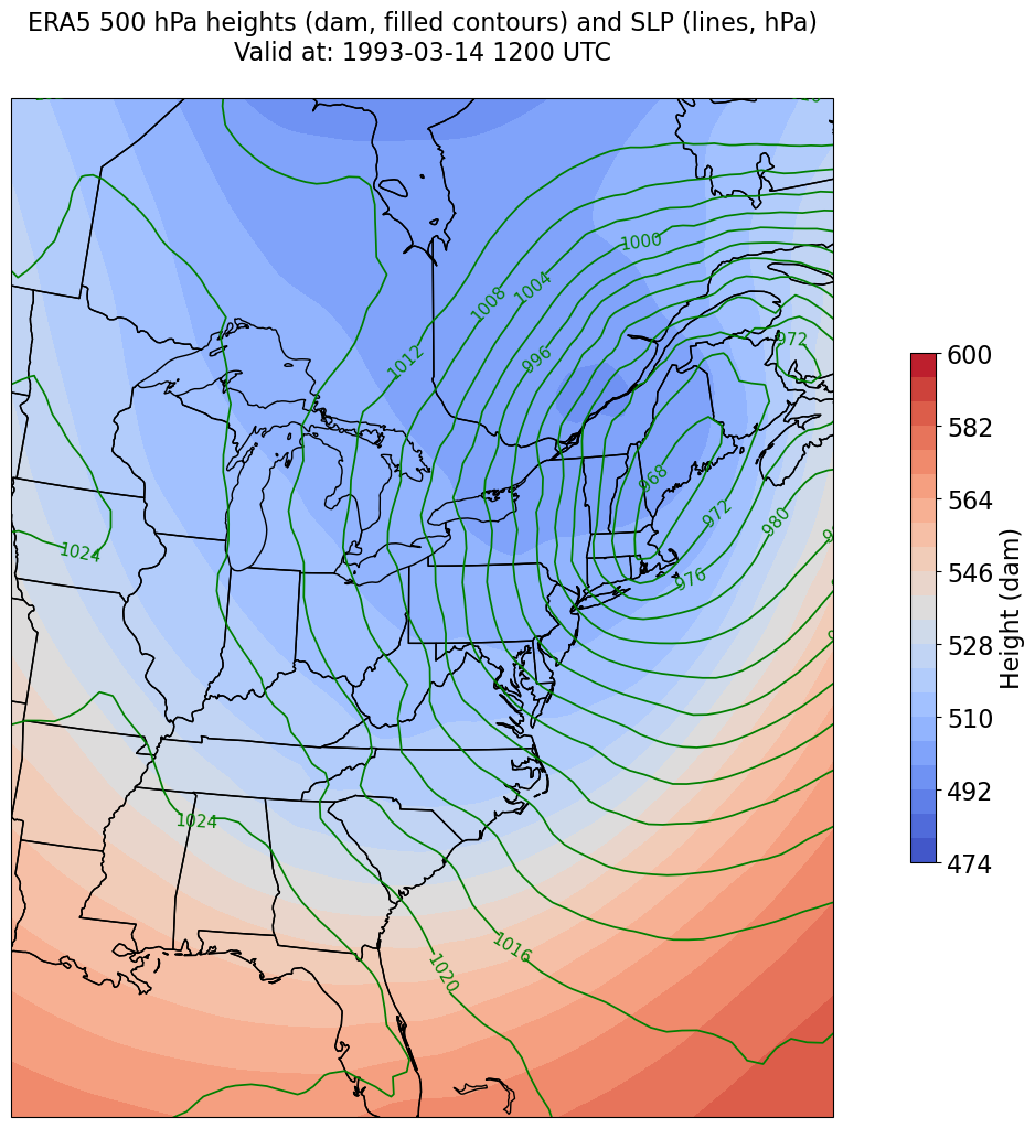
Plot the map, with filled contours of 500 hPa geopotential heights, and contour lines of SLP.#
Create a meaningful title string.
tl1 = f"ERA5 {levelStr} hPa heights (dam, filled contours) and SLP (lines, hPa)"
tl2 = f"Valid at: {timeStr}"
title_line = (tl1 + '\n' + tl2 + '\n')
proj_map = ccrs.LambertConformal(central_longitude=cLon, central_latitude=cLat)
proj_data = ccrs.PlateCarree()
res = '50m'
fig = plt.figure(figsize=(18,12))
ax = plt.subplot(1,1,1,projection=proj_map)
ax.set_extent ([lonW,lonE,latS,latN])
ax.add_feature(cfeature.COASTLINE.with_scale(res))
ax.add_feature(cfeature.STATES.with_scale(res))
CF = ax.contourf(lons,lats,z, levels=Zcintervals,transform=proj_data,cmap=plt.get_cmap('coolwarm'))
cbar = plt.colorbar(CF,shrink=0.5)
cbar.ax.tick_params(labelsize=16)
cbar.ax.set_ylabel("Height (dam)",fontsize=16)

CL = ax.contour(lons,lats,slp,SLPcintervals,transform=proj_data,linewidths=1.25,colors='green')
ax.clabel(CL, inline_spacing=0.2, fontsize=11, fmt='%.0f')
title = plt.title(title_line,fontsize=16)
We’re just missing the outer longitudes at higher latitudes. We could do one of two things to resolve this:
Re-subset our original datset by extending the longitudinal range
Slightly constrain the map plotting region
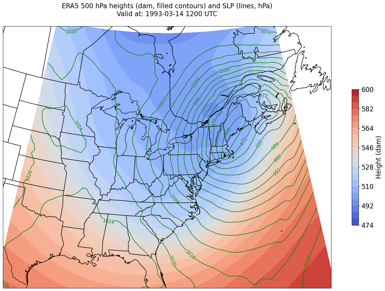
Let’s try the latter here.
constrainLon = 7 # trial and error!

proj_map = ccrs.LambertConformal(central_longitude=cLon, central_latitude=cLat)
proj_data = ccrs.PlateCarree()
res = '50m'
fig = plt.figure(figsize=(18,12))
ax = plt.subplot(1,1,1,projection=proj_map)
ax.set_extent ([lonW+constrainLon,lonE-constrainLon,latS,latN])
ax.add_feature(cfeature.COASTLINE.with_scale(res))
ax.add_feature(cfeature.STATES.with_scale(res))
CF = ax.contourf(lons,lats,z,levels=Zcintervals,transform=proj_data,cmap=plt.get_cmap('coolwarm'))
cbar = plt.colorbar(CF,shrink=0.5)
cbar.ax.tick_params(labelsize=16)
cbar.ax.set_ylabel("Height (dam)",fontsize=16)

CL = ax.contour(lons,lats,slp,SLPcintervals,transform=proj_data,linewidths=1.25,colors='green')
ax.clabel(CL, inline_spacing=0.2, fontsize=11, fmt='%.0f')
title = plt.title(title_line,fontsize=16)