04_Xarray: Overlays from a cloud-served ERA5 archive#
Overview#
Work with a cloud-served ERA5 archive
Subset the Dataset along its dimensions
Perform unit conversions
Create a well-labeled multi-parameter contour plot of gridded ERA5 data
Imports#
import xarray as xr
import pandas as pd
import numpy as np
from datetime import datetime as dt
from metpy.units import units
import metpy.calc as mpcalc
import cartopy.crs as ccrs
import cartopy.feature as cfeature
import matplotlib.pyplot as plt
Select the region, time, and (if applicable) vertical level(s) of interest.#
# Areal extent

lonW = -100
lonE = -60
latS = 25
latN = 55
cLat, cLon = (latS + latN)/2, (lonW + lonE)/2

# Recall that in ERA5, longitudes run between 0 and 360, not -180 and 180
if (lonW < 0 ):
    lonW = lonW + 360
if (lonE < 0 ):
    lonE = lonE + 360

expand = 1
latRange = np.arange(latS - expand,latN + expand,.25) # expand the data range a bit beyond the plot range
lonRange = np.arange((lonW - expand),(lonE + expand),.25) # Need to match longitude values to those of the coordinate variable

# Vertical level specificaton
plevel = 500
levelStr = str(plevel)

# Date/Time specification
Year = 1998
Month = 5
Day = 31
Hour = 18
Minute = 0
dateTime = dt(Year,Month,Day, Hour, Minute)
timeStr = dateTime.strftime("%Y-%m-%d %H%M UTC")
Work with a cloud-served ERA5 archive#
A team at Google Research & Cloud are making parts of the ECMWF Reanalysis version 5 (aka ERA-5) accessible in a Analysis Ready, Cloud Optimized (aka ARCO) format.
Access the ERA-5 ARCO catalog
The ERA5 archive runs from 1/1/1959 through 1/10/2023. For dates subsequent to the end-date, we’ll instead load a local archive.
If the requested date is later than 1/10/2023, read in the dataset from a locally-stored archive.#
endDate = dt(2023,1,10)
if (dateTime <= endDate):

    cloud_source = True
    ds = xr.open_dataset(
     'gs://weatherbench2/datasets/era5/1959-2023_01_10-wb13-6h-1440x721.zarr',
     chunks={'time': 48},
     consolidated=True,
     engine='zarr'
)

else:
    import glob, os
    cloud_source = False
    input_directory = '/free/ktyle/era5'
    files = glob.glob(os.path.join(input_directory,'*.nc'))
    ds = xr.open_mfdataset(files)

print(f'size: {ds.nbytes / (1024 ** 4)} TB')
size: 42.752324647717614 TB
The cloud-hosted dataset is a big (40+ TB) file! But Xarray is just reading only enough of the file for us to get a look at the dimensions, coordinate and data variables, and other metadata. We call this lazy loading, as opposed to eager loading, which we will do only after we have subset the dataset over time, lat-lon, and vertical level.
Examine the dataset#
ds
<xarray.Dataset> Size: 47TB
Dimensions:                                           (time: 93544,
                                                       latitude: 721,
                                                       longitude: 1440,
                                                       level: 13)
Coordinates:
  * latitude                                          (latitude) float32 3kB ...
  * level                                             (level) int64 104B 50 ....
  * longitude                                         (longitude) float32 6kB ...
  * time                                              (time) datetime64[ns] 748kB ...
Data variables: (12/50)
    10m_u_component_of_wind                           (time, latitude, longitude) float32 388GB dask.array<chunksize=(48, 721, 1440), meta=np.ndarray>
    10m_v_component_of_wind                           (time, latitude, longitude) float32 388GB dask.array<chunksize=(48, 721, 1440), meta=np.ndarray>
    2m_dewpoint_temperature                           (time, latitude, longitude) float32 388GB dask.array<chunksize=(48, 721, 1440), meta=np.ndarray>
    2m_temperature                                    (time, latitude, longitude) float32 388GB dask.array<chunksize=(48, 721, 1440), meta=np.ndarray>
    angle_of_sub_gridscale_orography                  (latitude, longitude) float32 4MB dask.array<chunksize=(721, 1440), meta=np.ndarray>
    anisotropy_of_sub_gridscale_orography             (latitude, longitude) float32 4MB dask.array<chunksize=(721, 1440), meta=np.ndarray>
    ...                                                ...
    v_component_of_wind                               (time, level, latitude, longitude) float32 5TB dask.array<chunksize=(48, 13, 721, 1440), meta=np.ndarray>
    vertical_velocity                                 (time, level, latitude, longitude) float32 5TB dask.array<chunksize=(48, 13, 721, 1440), meta=np.ndarray>
    volumetric_soil_water_layer_1                     (time, latitude, longitude) float32 388GB dask.array<chunksize=(48, 721, 1440), meta=np.ndarray>
    volumetric_soil_water_layer_2                     (time, latitude, longitude) float32 388GB dask.array<chunksize=(48, 721, 1440), meta=np.ndarray>
    volumetric_soil_water_layer_3                     (time, latitude, longitude) float32 388GB dask.array<chunksize=(48, 721, 1440), meta=np.ndarray>
volumetric_soil_water_layer_4 (time, latitude, longitude) float32 388GB dask.array<chunksize=(48, 721, 1440), meta=np.ndarray>Data variables selection and subsetting#
We’ll retrieve two data variables (i.e. DataArrays), geopotential and sea-level pressure, from the Dataset.
if (cloud_source):
    z = ds['geopotential'].sel(time=dateTime,level=plevel,latitude=latRange,longitude=lonRange)
    slp = ds['mean_sea_level_pressure'].sel(time=dateTime,latitude=latRange,longitude=lonRange)
else:
    z = ds['z'].sel(valid_time=dateTime,pressure_level=plevel,latitude=latRange,longitude=lonRange)
    slp = ds['msl'].sel(valid_time=dateTime,latitude=latRange,longitude=lonRange)
Define our subsetted coordinate arrays of lat and lon. Pull them from either of the two DataArrays. We’ll need to pass these into the contouring functions later on.#
lats = z.latitude
lons = z.longitude
Perform unit conversions#
Convert geopotential in m**2/s**2 to geopotential height in decameters (dam), and Pascals to hectoPascals (hPa).
We take the DataArrays and apply MetPy’s unit conversion methods.
slp = slp.metpy.convert_units('hPa')
z = mpcalc.geopotential_to_height(z).metpy.convert_units('dam')
slp.nbytes / 1e6, z.nbytes / 1e6 # size in MB for the subsetted DataArrays
(0.086016, 0.086016)
z
<xarray.DataArray 'truediv-bd78aa20df4aa91642e81348ecc231b3' (latitude: 128,
                                                              longitude: 168)> Size: 86kB
<Quantity(dask.array<mul, shape=(128, 168), dtype=float32, chunksize=(128, 168), chunktype=numpy.ndarray>, 'decameter')>
Coordinates:
  * latitude   (latitude) float32 512B 24.0 24.25 24.5 ... 55.25 55.5 55.75
    level      int64 8B 500
  * longitude  (longitude) float32 672B 259.0 259.2 259.5 ... 300.2 300.5 300.8
time datetime64[ns] 8B 1998-05-31T18:00:00Create a well-labeled multi-parameter contour plot of gridded ERA5 reanalysis data#
We will make contour fills of 500 hPa height in decameters, with a contour interval of 6 dam, and contour lines of SLP in hPa, contour interval = 4.
As we’ve done before, let’s first define some variables relevant to Cartopy. Recall that we already defined the areal extent up above when we did the data subsetting.
proj_map = ccrs.LambertConformal(central_longitude=cLon, central_latitude=cLat)
proj_data = ccrs.PlateCarree() # Our data is lat-lon; thus its native projection is Plate Carree.
res = '50m'
Now define the range of our contour values and a contour interval. 60 m is standard for 500 hPa.#
minVal = 474
maxVal = 606
cint = 6
Zcintervals = np.arange(minVal, maxVal, cint)
Zcintervals
array([474, 480, 486, 492, 498, 504, 510, 516, 522, 528, 534, 540, 546,
       552, 558, 564, 570, 576, 582, 588, 594, 600])
minVal = 900
maxVal = 1080
cint = 4
SLPcintervals = np.arange(minVal, maxVal, cint)
SLPcintervals
array([ 900,  904,  908,  912,  916,  920,  924,  928,  932,  936,  940,
        944,  948,  952,  956,  960,  964,  968,  972,  976,  980,  984,
        988,  992,  996, 1000, 1004, 1008, 1012, 1016, 1020, 1024, 1028,
       1032, 1036, 1040, 1044, 1048, 1052, 1056, 1060, 1064, 1068, 1072,
       1076])
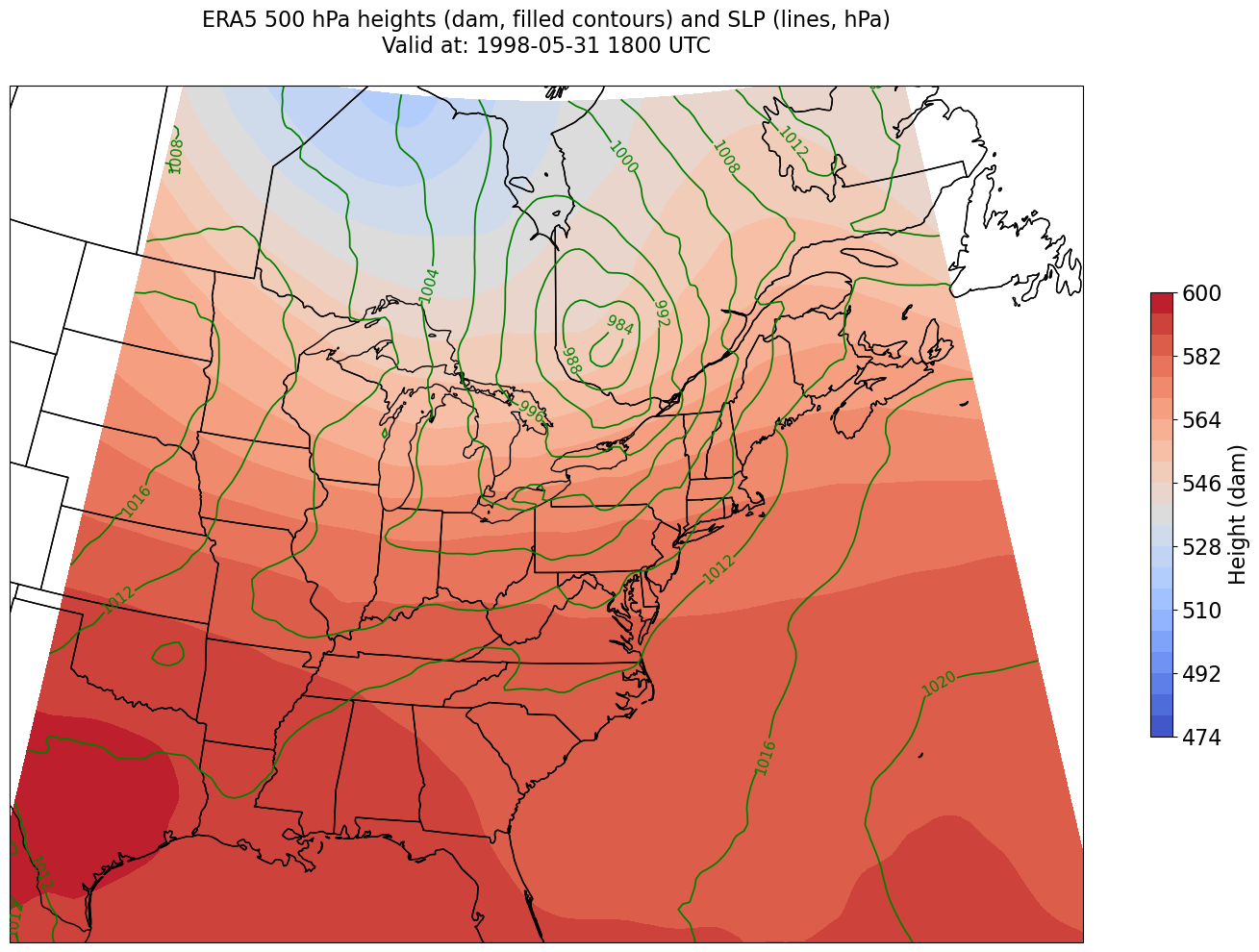
Plot the map, with filled contours of 500 hPa geopotential heights, and contour lines of SLP.#
Create a meaningful title string.
tl1 = f"ERA5 {levelStr} hPa heights (dam, filled contours) and SLP (lines, hPa)"
tl2 = f"Valid at: {timeStr}"
title_line = (tl1 + '\n' + tl2 + '\n')
proj_map = ccrs.LambertConformal(central_longitude=cLon, central_latitude=cLat)
proj_data = ccrs.PlateCarree()
res = '50m'
fig = plt.figure(figsize=(18,12))
ax = plt.subplot(1,1,1,projection=proj_map)
ax.set_extent ([lonW,lonE,latS,latN])
ax.add_feature(cfeature.COASTLINE.with_scale(res))
ax.add_feature(cfeature.STATES.with_scale(res))
CF = ax.contourf(lons,lats,z, levels=Zcintervals,transform=proj_data,cmap=plt.get_cmap('coolwarm'))
cbar = plt.colorbar(CF,shrink=0.5)
cbar.ax.tick_params(labelsize=16)
cbar.ax.set_ylabel("Height (dam)",fontsize=16)

CL = ax.contour(lons,lats,slp,SLPcintervals,transform=proj_data,linewidths=1.25,colors='green')
ax.clabel(CL, inline_spacing=0.2, fontsize=11, fmt='%.0f')
title = plt.title(title_line,fontsize=16)
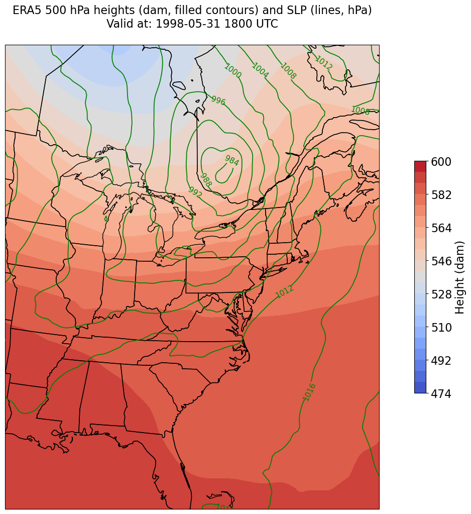
Constrain the map plotting region to eliminate blank space on the east & west edges of the domain.#
constrainLon = 7 # trial and error!

proj_map = ccrs.LambertConformal(central_longitude=cLon, central_latitude=cLat)
proj_data = ccrs.PlateCarree()
res = '50m'
fig = plt.figure(figsize=(18,12))
ax = plt.subplot(1,1,1,projection=proj_map)
ax.set_extent ([lonW+constrainLon,lonE-constrainLon,latS,latN])
ax.add_feature(cfeature.COASTLINE.with_scale(res))
ax.add_feature(cfeature.STATES.with_scale(res))
CF = ax.contourf(lons,lats,z,levels=Zcintervals,transform=proj_data,cmap=plt.get_cmap('coolwarm'))
cbar = plt.colorbar(CF,shrink=0.5)
cbar.ax.tick_params(labelsize=16)
cbar.ax.set_ylabel("Height (dam)",fontsize=16)

CL = ax.contour(lons,lats,slp,SLPcintervals,transform=proj_data,linewidths=1.25,colors='green')
ax.clabel(CL, inline_spacing=0.2, fontsize=11, fmt='%.0f')
title = plt.title(title_line,fontsize=16)
Things to try:#
Change the date and time
Change the region
Use a different map projection for your plot
Select and overlay different variables