MetPy Intro: NYS Mesonet Map#
Overview#
In this notebook, we’ll use Cartopy, Matplotlib, and Pandas (with a bunch of help from MetPy) to read in, manipulate, and visualize current data from the New York State Mesonet.
Prerequisites#
Concepts |
Importance |
Notes |
|---|---|---|
Matplotlib |
Necessary |
|
Cartopy |
Necessary |
|
Pandas |
Necessary |
|
MetPy |
Necessary |
Intro |
Time to learn: 30 minutes
Imports#
import matplotlib.pyplot as plt
import numpy as np
import pandas as pd
from datetime import datetime
from cartopy import crs as ccrs
from cartopy import feature as cfeature
from metpy.calc import wind_components, dewpoint_from_relative_humidity
from metpy.units import units
from metpy.plots import StationPlot, USCOUNTIES
Create a Pandas DataFrame object pointing to the most recent set of NYSM obs.
nysm_data = pd.read_csv('https://www.atmos.albany.edu/products/nysm/nysm_latest.csv')
nysm_data.columns
Index(['station', 'time', 'temp_2m [degC]', 'temp_9m [degC]',
       'relative_humidity [percent]', 'precip_incremental [mm]',
       'precip_local [mm]', 'precip_max_intensity [mm/min]',
       'avg_wind_speed_prop [m/s]', 'max_wind_speed_prop [m/s]',
       'wind_speed_stddev_prop [m/s]', 'wind_direction_prop [degrees]',
       'wind_direction_stddev_prop [degrees]', 'avg_wind_speed_sonic [m/s]',
       'max_wind_speed_sonic [m/s]', 'wind_speed_stddev_sonic [m/s]',
       'wind_direction_sonic [degrees]',
       'wind_direction_stddev_sonic [degrees]', 'solar_insolation [W/m^2]',
       'station_pressure [mbar]', 'snow_depth [cm]', 'frozen_soil_05cm [bit]',
       'frozen_soil_25cm [bit]', 'frozen_soil_50cm [bit]',
       'soil_temp_05cm [degC]', 'soil_temp_25cm [degC]',
       'soil_temp_50cm [degC]', 'soil_moisture_05cm [m^3/m^3]',
       'soil_moisture_25cm [m^3/m^3]', 'soil_moisture_50cm [m^3/m^3]', 'lat',
       'lon', 'elevation', 'name'],
      dtype='object')
Create several Series objects for some of the columns.
stid = nysm_data['station']
lats = nysm_data['lat']
lons = nysm_data['lon']
Our goal is to make a map of NYSM observations, which includes the wind velocity. The convention is to plot wind velocity using wind barbs. The MetPy library allows us to not only make such a map, but perform a variety of meteorologically-relevant calculations and diagnostics. Here, we will use such a calculation, which will determine the two scalar components of wind velocity (u and v), from wind speed and direction. We will use MetPy’s wind_components method.
This method requires us to do the following:
Create Pandas
Seriesobjects for the variables of interestExtract the underlying Numpy array via the
Series’valuesattributeAttach units to these arrays using MetPy’s
unitsclass
Perform these three steps#
wspd = nysm_data['max_wind_speed_prop [m/s]'].values * units['m/s']
drct = nysm_data['wind_direction_prop [degrees]'].values * units['degree']
Examine these two units aware Series
wspd
| Magnitude | [7.5 4.6 18.5 5.6 9.3 9.5 11.1 4.4 11.5 4.9 nan 5.8 12.6 4.9 4.3 2.5 9.5 10.1 11.9 5.2 9.5 8.4 2.2 5.3 6.5 15.3 10.4 13.0 15.0 8.6 10.5 10.5 7.0 5.4 13.3 4.3 1.8 7.7 17.0 2.6 12.3 1.1 10.9 13.6 9.1 8.1 15.3 8.9 3.6 11.8 7.1 15.1 20.1 11.6 11.9 20.6 6.2 6.1 3.8 2.1 7.8 8.6 8.2 12.7 14.7 11.3 3.8 11.4 10.0 5.9 6.3 1.7 3.7 3.3 8.4 12.0 4.9 3.2 4.8 8.1 9.0 7.2 15.5 8.5 13.6 5.2 8.6 2.5 7.0 9.8 12.2 10.5 3.7 12.8 3.2 9.2 4.7 7.4 4.4 7.6 9.4 10.1 8.7 8.7 8.1 5.1 nan 8.5 10.0 6.4 9.2 11.6 8.0 2.0 6.1 7.0 15.5 6.9 5.9 3.7 10.6 6.9 13.4 1.8 5.1 4.7 17.0] |
|---|---|
| Units | meter/second |
drct
| Magnitude | [219.0 188.0 244.0 228.0 246.0 189.0 205.0 168.0 225.0 223.0 nan 189.0 240.0 228.0 218.0 308.0 223.0 226.0 226.0 184.0 220.0 165.0 96.0 191.0 217.0 267.0 250.0 211.0 237.0 216.0 211.0 222.0 222.0 189.0 249.0 198.0 241.0 243.0 245.0 230.0 220.0 204.0 243.0 233.0 179.0 195.0 246.0 223.0 213.0 207.0 235.0 247.0 225.0 243.0 210.0 233.0 247.0 186.0 202.0 256.0 205.0 203.0 224.0 233.0 225.0 229.0 249.0 220.0 243.0 174.0 146.0 69.0 238.0 174.0 227.0 243.0 240.0 194.0 207.0 215.0 217.0 213.0 221.0 224.0 230.0 192.0 253.0 195.0 187.0 174.0 247.0 257.0 114.0 247.0 216.0 183.0 217.0 179.0 186.0 214.0 223.0 218.0 220.0 224.0 191.0 220.0 nan 279.0 178.0 188.0 231.0 230.0 131.0 274.0 234.0 227.0 245.0 267.0 198.0 199.0 224.0 220.0 253.0 252.0 171.0 268.0 252.0] |
|---|---|
| Units | degree |
Convert wind speed from m/s to knots
wspk = wspd.to('knots')
wspk
| Magnitude | [14.578833693304537 8.941684665226783 35.96112311015119 10.885529157667387 18.077753779697627 18.466522678185747 21.57667386609071 8.552915766738662 22.354211663066955 9.524838012958964 nan 11.274298056155509 24.49244060475162 9.524838012958964 8.3585313174946 4.859611231101512 18.466522678185747 19.632829373650107 23.1317494600432 10.107991360691146 18.466522678185747 16.32829373650108 4.276457883369331 10.302375809935205 12.63498920086393 29.740820734341256 20.215982721382293 25.26997840172786 29.157667386609074 16.7170626349892 20.41036717062635 20.41036717062635 13.606911447084235 10.496760259179267 25.853131749460047 8.3585313174946 3.4989200863930887 14.967602591792657 33.045356371490286 5.053995680345573 23.90928725701944 2.1382289416846656 21.187904967602595 26.436285097192226 17.688984881209503 15.745140388768899 29.740820734341256 17.300215982721383 6.997840172786177 22.937365010799137 13.801295896328293 29.352051835853132 39.07127429805616 22.548596112311017 23.1317494600432 40.04319654427646 12.05183585313175 11.857451403887689 7.386609071274298 4.08207343412527 15.161987041036717 16.7170626349892 15.939524838012959 24.68682505399568 28.57451403887689 21.965442764578835 7.386609071274298 22.159827213822897 19.43844492440605 11.468682505399569 12.24622030237581 3.304535637149028 7.192224622030238 6.4146868250539955 16.32829373650108 23.326133909287257 9.524838012958964 6.220302375809936 9.330453563714903 15.745140388768899 17.494600431965445 13.995680345572355 30.129589632829376 16.522678185745143 26.436285097192226 10.107991360691146 16.7170626349892 4.859611231101512 13.606911447084235 19.04967602591793 23.714902807775378 20.41036717062635 7.192224622030238 24.881209503239745 6.220302375809936 17.883369330453565 9.136069114470843 14.384449244060477 8.552915766738662 14.773218142548597 18.272138228941685 19.632829373650107 16.91144708423326 16.91144708423326 15.745140388768899 9.913606911447085 nan 16.522678185745143 19.43844492440605 12.440604751619873 17.883369330453565 22.548596112311017 15.550755939524839 3.8876889848812097 11.857451403887689 13.606911447084235 30.129589632829376 13.412526997840175 11.468682505399569 7.192224622030238 20.60475161987041 13.412526997840175 26.047516198704106 3.4989200863930887 9.913606911447085 9.136069114470843 33.045356371490286] |
|---|---|
| Units | knot |
Perform the vector decomposition#
u, v = wind_components(wspk, drct)
Take a look at one of the output components:
u
| Magnitude | [9.174757320920959 1.2444419826666766 32.321643349635266 8.089524666103818 16.514849849824127 2.888800596315276 9.11869640343323 -1.7782511784845076 15.806814655034053 6.49592390469896 nan 1.7636887851188001 21.211075764396398 7.078334082840842 5.146025722484443 3.829425908455992 12.594138182579615 14.122675561724275 16.639588038071178 0.705097833957897 11.870051971533286 -4.226073393034684 -4.253030999631061 1.9657859782853526 7.603926318443808 29.70006197315439 18.996809785218367 13.015001029044566 24.4536774670912 9.826042878496201 10.512116215766765 13.657201360888145 9.104800907258763 1.6420550758002623 24.135977764949256 2.5829282251210497 3.0602244612652734 13.336231560745981 29.949263804882825 3.8715853064760446 15.368593605248359 0.8696960618683418 18.87856156001704 21.11295603235176 -0.30871535360983016 4.075142200426299 27.16959168842034 11.798718928943007 3.8112969188956543 10.413345803961093 11.305359747314592 27.01870617369042 27.627563005755174 20.090946247357582 11.565874730021601 31.979918696062224 11.093773395819907 1.2394411735192608 2.7670724610851387 3.96081840747653 6.4077326078179455 6.5318767483952 11.072524349864796 19.71577511844613 20.205232646000052 16.577530088262616 6.895993647128358 14.244062365839943 17.319781247722055 -1.1988037579940418 -6.847999487427938 -3.085049789504792 6.099352397842114 -0.6705173561661589 11.941758065315181 20.78373749726646 8.248751686154154 1.5048273419590552 4.235937276187563 9.03104151403699 10.528513363999119 7.6225938377913085 19.766789318396487 11.477616704128144 20.251369295413152 2.101569574572602 15.986606503572125 1.257759938403179 1.6582653638281386 -1.991233360735866 21.829683133710137 19.887250782333634 -6.570424133800996 22.903274107499165 3.6562020013009127 0.9359432347550167 5.498223645643984 -0.25104325458381793 0.8940231415548767 8.26107874673846 12.461568306973513 12.087176696998343 10.870468647614691 11.747678273637039 3.004314419643652 6.372343689981027 nan 16.3192565994661 -0.678391944541059 1.7313975411014633 13.897988252405435 17.273226751970043 -11.736304487265572 3.8782187699086044 9.592879695720217 9.951465054429319 27.306681704451986 13.394145595736294 3.544017797259115 2.3415592966357064 14.313263183971564 8.62140616879786 24.90936362184494 3.3276707481601484 -1.550829793811361 9.130503668014633 31.428001510401405] |
|---|---|
| Units | knot |
# Write your code here
nysm_data['temp_2m [degC]']
0      20.6
1      17.1
2      16.6
3      18.8
4      18.6
       ...
122    16.2
123    14.4
124    12.7
125    18.1
126    20.0
Name: temp_2m [degC], Length: 127, dtype: float64
# %load /spare11/atm350/common/mar25/metpy1.py
tmpc = nysm_data['temp_2m [degC]'].values * units('degC')
tmpf = tmpc.to('degF')
Now, let’s plot several of the meteorological values on a map. We will use Matplotlib and Cartopy, as well as MetPy’s StationPlot method.
Create units-aware objects for relative humidity and station pressure
rh = nysm_data['relative_humidity [percent]'].values * units('percent')
pres = nysm_data['station_pressure [mbar]'].values * units('mbar')
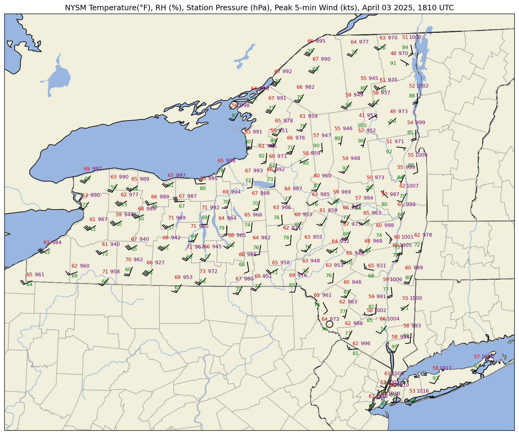
Plot the map, centered over NYS, with add some geographic features, and the mesonet data.#
Determine the current time, for use in the plot’s title and a version to be saved to disk.
timeString = nysm_data['time'][0]
timeObj = datetime.strptime(timeString,"%Y-%m-%d %H:%M:%S")
titleString = datetime.strftime(timeObj,"%B %d %Y, %H%M UTC")
figString = datetime.strftime(timeObj,"%Y%m%d_%H%M")
Previously, we used the ax.scatter and ax.text methods to plot markers for the stations and their site id’s. The latter method does not provide an intuitive means to orient several text stings relative to a central point as we typically do for a meteorological surface station plot. Let’s take advantage of the Metpy package, and its StationPlot method!#
Be patient: this may take a minute or so to plot, if you chose the highest resolution for the shapefiles!#
Specify two resolutions: one for the Natural Earth shapefiles, and the other for MetPy’s US County shapefiles.#
res = '10m'
resCounty = '5m'
# Set the domain for defining the plot region.
latN = 45.2
latS = 40.2
lonW = -80.0
lonE = -72.0
cLat = (latN + latS)/2
cLon = (lonW + lonE )/2

proj = ccrs.LambertConformal(central_longitude=cLon, central_latitude=cLat)

fig = plt.figure(figsize=(18,12),dpi=150) # Increase the dots per inch from default 100 to make plot easier to read
ax = fig.add_subplot(1,1,1,projection=proj)
ax.set_extent ([lonW,lonE,latS,latN])
ax.set_facecolor(cfeature.COLORS['water'])
ax.add_feature (cfeature.STATES.with_scale(res))
ax.add_feature (cfeature.RIVERS.with_scale(res))
ax.add_feature (cfeature.LAND.with_scale(res))
ax.add_feature (cfeature.COASTLINE.with_scale(res))
ax.add_feature (cfeature.LAKES.with_scale(res))
ax.add_feature (cfeature.STATES.with_scale(res))

ax.add_feature(USCOUNTIES.with_scale(resCounty), linewidth=0.8, edgecolor='darkgray')

# Create a station plot pointing to an Axes to draw on as well as the location of points
stationplot = StationPlot(ax, lons, lats, transform=ccrs.PlateCarree(),
                          fontsize=8)

stationplot.plot_parameter('NW', tmpf, color='red')
stationplot.plot_parameter('SW', rh, color='green')
stationplot.plot_parameter('NE', pres, color='purple')
stationplot.plot_barb(u, v,zorder=2) # zorder value set so wind barbs will display over lake features

plotTitle = f'NYSM Temperature(°F), RH (%), Station Pressure (hPa), Peak 5-min Wind (kts), {titleString}'
ax.set_title (plotTitle);
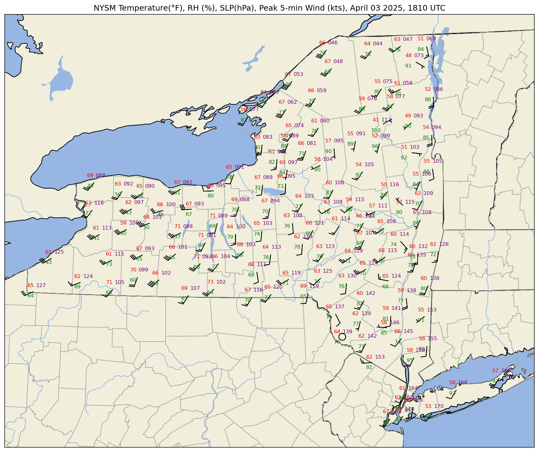
What if we wanted to plot sea-level pressure (SLP) instead of station pressure? In this case, we can apply what’s called a reduction to sea-level pressure formula. This formula requires station elevation (accounting for sensor height) in meters, temperature in Kelvin, and station pressure in hectopascals. We assume each NYSM station has its sensor height .5 meters above ground level.
pres.m
array([ 952.65,  952.96,  977.28, 1003.77,  957.61,  991.22,  962.1 ,
        965.71,  950.55, 1012.93,     nan,  993.28,  988.81, 1009.43,
        953.27,  997.03,  989.95,  945.42,  997.49,  991.81,  997.64,
        999.97,  970.64,  962.11,  946.45,  986.9 ,  960.51,  972.64,
        941.69,  960.2 ,  988.95,  978.39,  959.27,  992.72,  939.73,
        975.84,  999.75,  962.57,  967.2 ,  972.74,  981.68,  973.24,
        970.01,  972.04, 1001.81,  988.43,  984.33,  944.95,  998.72,
        978.31,  965.1 ,  939.86,  992.16,  951.9 ,  951.3 ,  927.39,
        985.19,  991.07,  951.6 ,  984.03,  994.44, 1004.74,  954.8 ,
        936.52,  994.55,  976.86, 1005.23,  990.04,  967.57,  966.44,
        960.81,  950.66,  973.39,  947.21,  958.28,  997.45,  969.12,
        970.59,  997.98,  986.22,  960.05,  980.14,  990.89,  947.65,
        989.76, 1009.99,  960.14,  945.99,  964.73, 1005.96,  945.54,
        988.78,  969.63,  968.69,  999.12, 1000.61, 1007.08,  964.12,
        970.65,  993.62, 1015.73,  987.3 ,  959.  , 1012.37,  978.49,
       1011.45,     nan,  931.28,  999.27,  966.41,  949.29,  967.17,
        997.71, 1001.58,  947.89, 1015.92,  947.72,  995.81,  991.94,
        963.34,  995.99,  986.86,  935.35,  958.53, 1005.99,  995.18,
        989.29])
elev = nysm_data['elevation']
sensorHeight = .5
# Reduce station pressure to SLP. Source: https://www.sandhurstweather.org.uk/barometric.pdf
slp = pres.m/np.exp(-1*(elev+sensorHeight)/((tmpc.m + 273.15) * 29.263))
slp
0      1010.659178
1      1012.980443
2      1009.688866
3      1014.478484
4      1011.908947
          ...
122    1005.826914
123    1010.401427
124    1010.457341
125    1009.494629
126    1010.083936
Name: elevation, Length: 127, dtype: float64
Make a new map, substituting SLP for station pressure. We will also use the convention of the three least-significant digits to represent SLP in hectopascals.
fig = plt.figure(figsize=(18,12),dpi=150) # Increase the dots per inch from default 100 to make plot easier to read
ax = fig.add_subplot(1,1,1,projection=proj)
ax.set_extent ([lonW,lonE,latS,latN])
ax.set_facecolor(cfeature.COLORS['water'])
ax.add_feature (cfeature.STATES.with_scale(res))
ax.add_feature (cfeature.RIVERS.with_scale(res))
ax.add_feature (cfeature.LAND.with_scale(res))
ax.add_feature (cfeature.COASTLINE.with_scale(res))
ax.add_feature (cfeature.LAKES.with_scale(res))
ax.add_feature (cfeature.STATES.with_scale(res))

ax.add_feature(USCOUNTIES.with_scale(resCounty), linewidth=0.8, edgecolor='darkgray')

stationplot = StationPlot(ax, lons, lats, transform=ccrs.PlateCarree(),
                          fontsize=8)

stationplot.plot_parameter('NW', tmpf, color='red')
stationplot.plot_parameter('SW', rh, color='green')
# A more complex example uses a custom formatter to control how the sea-level pressure
# values are plotted. This uses the standard trailing 3-digits of the pressure value
# in tenths of millibars.
stationplot.plot_parameter('NE', slp, color='purple', formatter=lambda v: format(10 * v, '.0f')[-3:])
stationplot.plot_barb(u, v,zorder=2)
plotTitle = f'NYSM Temperature(°F), RH (%), SLP(hPa), Peak 5-min Wind (kts), {titleString}'
ax.set_title (plotTitle);
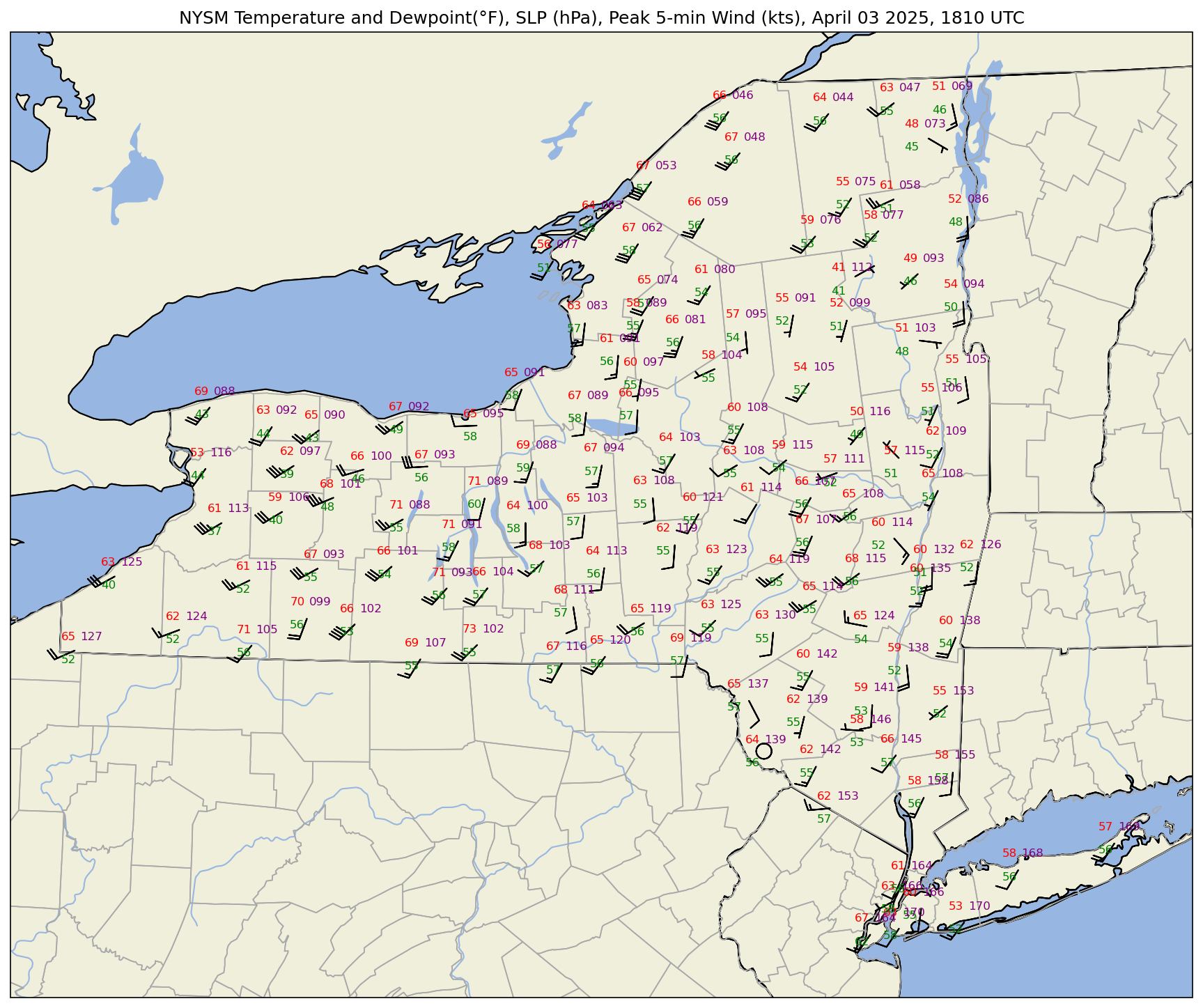
One last thing to do … plot dewpoint instead of RH. MetPy’s dewpoint_from_relative_humidity takes care of this!
dwpc = dewpoint_from_relative_humidity(tmpf, rh)
dwpc
| Magnitude | [12.848088759964355 12.879292733049851 3.940983397577895 14.030254830591616 13.308135433966356 14.091187025371482 13.279937597932587 13.751840282730655 13.552489408612075 14.312729167520558 nan 13.706279567454885 5.836163830149417 13.513731525147591 12.928612701882571 10.58397735143933 6.726411664734371 13.767659212719025 6.2852472753514235 13.895204759978753 10.30539456984394 7.842190558849779 9.00940128322543 13.572685352241479 12.730577091728719 13.188903691266603 11.212759138338242 13.2570329941571 12.230895917287455 12.785975738340085 11.950821077591229 13.83107635643637 12.460163765897391 14.56872272660462 11.131719431103136 13.844080950949035 11.384758475870456 13.091818743357692 2.9722670114725815 9.590806106580374 13.108222876637342 13.419668264311667 12.702186976022233 12.81081983130673 8.991585338621348 14.124017551629208 4.336201204686745 10.934484430509826 10.316782293111544 13.521654505231197 13.661262851908418 12.727748455009078 13.630887880996909 12.540066384157683 12.825439357292112 11.899288690394656 12.835064271980002 11.595899082595054 10.5703629478935 11.109047567223456 15.052463588137812 10.917991667425667 12.9393333078458 10.913662475096942 13.24794673877983 13.383325074965057 14.719434620298046 6.8372081304096355 13.274783045677736 12.951973617243823 13.903400178741094 4.771316482782879 7.975523299832787 12.138281803700579 13.408283081774357 9.316865218960686 12.186111194328817 12.932845701307997 14.40106389855083 12.69086603701868 14.035902165704215 14.622225127387651 14.342387551737204 10.906449502734176 13.60596591140336 12.776657967722372 10.937176775792238 11.033110681744972 13.06571172992659 11.061382062672521 12.634266279280325 7.535412905789485 7.428470102039398 12.739129011058935 12.106592308651273 10.746278915513471 11.119685489449466 14.384601882293907 12.98341372890377 13.443002097663395 13.300548436361737 13.457024867327675 nan 16.488949447493212 11.334022929481534 13.34881409016873 nan 12.268867724188567 9.771533451276468 13.886331684360812 11.680134162405125 13.408283081774357 11.026253541135532 11.91193928144861 13.032660881370475 11.325571796940892 4.715679427842872 13.677745047375026 15.488386737117594 12.554389202508673 12.949088546900214 13.850960056733754 10.748380601282804 12.832315459656002 10.713285340980576 14.598357490563046 9.150867407154067] |
|---|---|
| Units | degree_Celsius |
The dewpoint is returned in units of degrees Celsius, so convert to Fahrenheit.
dwpf = dwpc.to('degF')
Plot the map
res = '10m'
fig = plt.figure(figsize=(18,12),dpi=150) # Increase the dots per inch from default 100 to make plot easier to read
ax = fig.add_subplot(1,1,1,projection=proj)
ax.set_extent ([lonW,lonE,latS,latN])
ax.set_facecolor(cfeature.COLORS['water'])
ax.add_feature(cfeature.STATES.with_scale(res))
ax.add_feature(cfeature.RIVERS.with_scale(res))
ax.add_feature (cfeature.LAND.with_scale(res))
ax.add_feature(cfeature.COASTLINE.with_scale(res))
ax.add_feature (cfeature.LAKES.with_scale(res))
ax.add_feature (cfeature.STATES.with_scale(res))

ax.add_feature(USCOUNTIES.with_scale(resCounty), linewidth=0.8, edgecolor='darkgray')

stationplot = StationPlot(ax, lons, lats, transform=ccrs.PlateCarree(),
                          fontsize=8)

stationplot.plot_parameter('NW', tmpf, color='red')
stationplot.plot_parameter('SW', dwpf, color='green')
# A more complex example uses a custom formatter to control how the sea-level pressure
# values are plotted. This uses the standard trailing 3-digits of the pressure value
# in tenths of millibars.
stationplot.plot_parameter('NE', slp, color='purple', formatter=lambda v: format(10 * v, '.0f')[-3:])
stationplot.plot_barb(u, v,zorder=2)
plotTitle = f'NYSM Temperature and Dewpoint(°F), SLP (hPa), Peak 5-min Wind (kts), {titleString}'
ax.set_title (plotTitle);
Save the plot to the current directory.
figName = f'NYSM_{figString}.png'
figName
'NYSM_20250403_1810.png'
fig.savefig(figName)
Summary#
The MetPy library provides methods to assign physical units to numerical arrays and perform units-aware calculations
MetPy’s
StationPlotmethod offers a customized use of Matplotlib’s Pyplot library to plot several meteorologically-relevant parameters centered about several geo-referenced points.
What’s Next?#
In the next notebook, we will plot METAR observations from sites across the world, using a different access method to retrieve the data.