Skew-T’s#
Requesting Upper Air Data from Siphon and Plotting a Skew-T with MetPy#
Based on Unidata’s MetPy Monday # 15 -17 YouTube links:
https://www.youtube.com/watch?v=OUTBiXEuDIU;
https://www.youtube.com/watch?v=oog6_b-844Q;
https://www.youtube.com/watch?v=b0RsN9mCY5k#
Import the libraries we need#
import numpy as np
import matplotlib.pyplot as plt
import matplotlib.gridspec as gridspec
from mpl_toolkits.axes_grid1.inset_locator import inset_axes
import metpy.calc as mpcalc
from metpy.plots import Hodograph, SkewT
from metpy.units import units, pandas_dataframe_to_unit_arrays
from datetime import datetime, timedelta
import pandas as pd
from siphon.simplewebservice.wyoming import WyomingUpperAir
Next we use methods from the datetime library to determine the latest time, and then use it to select the most recent date and time that we’ll use for our selected Skew-T.#
now = datetime.now()

curr_year = now.year
curr_month = now.month
curr_day = now.day
curr_hour = now.hour

print(f"Current time is: {now}")
print(f"Current year, month, date, hour: {curr_year}, {curr_month}, {curr_day}, {curr_hour}")

if (curr_hour > 13) :
    raob_hour = 12
    hr_delta = curr_hour - 12
elif (curr_hour > 1):
    raob_hour = 0
    hr_delta = curr_hour - 0
else:
    raob_hour = 12
    hr_delta = curr_hour + 12

raob_time = now - timedelta(hours=hr_delta)

raob_year = raob_time.year
raob_month = raob_time.month
raob_day = raob_time.day
raob_hour = raob_time.hour

print(f"Time of RAOB is: {raob_year}, {raob_month}, {raob_day}, {raob_hour}")
Current time is: 2025-04-08 16:36:22.801816
Current year, month, date, hour: 2025, 4, 8, 16
Time of RAOB is: 2025, 4, 8, 12
Construct a datetime object that we will use in our query to the data server. Note what it looks like.#
query_date = datetime(raob_year,raob_month,raob_day,raob_hour)
query_date
datetime.datetime(2025, 4, 8, 12, 0)
If desired, we can choose a past date and time.#
#current = True
current = False
if (current == False):
    query_date = datetime(2025, 4, 2, 18)

raob_timeStr = query_date.strftime("%Y-%m-%d %H UTC")
raob_timeTitle = query_date.strftime("%H00 UTC %-d %b %Y")
print(raob_timeStr)
print(raob_timeTitle)
2025-04-02 18 UTC
1800 UTC 2 Apr 2025
Select our station and query the data server.#
station = 'ILX'

df = WyomingUpperAir.request_data (query_date,station)
- If you get a
No data available for YYYY-MM-DD HHZ for station XXX, you may have specified an incorrect date or location, or there just might not have been a successful RAOB at that date and time. - If you get a
503 Server Error, try requesting the sounding again. The Wyoming server does not handle simultaneous requests well. Usually the request will eventually work.
What does the returned data file look like? Well, it looks like a Pandas Dataframe!#
df
| pressure | height | temperature | dewpoint | direction | speed | u_wind | v_wind | station | station_number | time | latitude | longitude | elevation | pw | |
|---|---|---|---|---|---|---|---|---|---|---|---|---|---|---|---|
| 0 | 977.0 | 178 | 23.6 | 18.6 | 180.0 | 16.0 | -1.959435e-15 | 16.000000 | ILX | 74560 | 2025-04-02 18:00:00 | 40.15 | -89.33 | 178.0 | 35.97 |
| 1 | 957.0 | 359 | 22.0 | 16.2 | 185.0 | 28.0 | 2.440361e+00 | 27.893452 | ILX | 74560 | 2025-04-02 18:00:00 | 40.15 | -89.33 | 178.0 | 35.97 |
| 2 | 954.0 | 387 | 21.8 | 15.8 | 186.0 | 29.0 | 3.031325e+00 | 28.841135 | ILX | 74560 | 2025-04-02 18:00:00 | 40.15 | -89.33 | 178.0 | 35.97 |
| 3 | 931.0 | 599 | 20.1 | 15.2 | 195.0 | 40.0 | 1.035276e+01 | 38.637033 | ILX | 74560 | 2025-04-02 18:00:00 | 40.15 | -89.33 | 178.0 | 35.97 |
| 4 | 925.0 | 655 | 19.6 | 15.0 | 195.0 | 42.0 | 1.087040e+01 | 40.568885 | ILX | 74560 | 2025-04-02 18:00:00 | 40.15 | -89.33 | 178.0 | 35.97 |
| ... | ... | ... | ... | ... | ... | ... | ... | ... | ... | ... | ... | ... | ... | ... | ... |
| 227 | 8.4 | 31889 | -44.3 | -67.3 | 290.0 | 17.0 | 1.597477e+01 | -5.814342 | ILX | 74560 | 2025-04-02 18:00:00 | 40.15 | -89.33 | 178.0 | 35.97 |
| 228 | 8.0 | 32218 | -43.1 | -66.6 | 290.0 | 14.0 | 1.315570e+01 | -4.788282 | ILX | 74560 | 2025-04-02 18:00:00 | 40.15 | -89.33 | 178.0 | 35.97 |
| 229 | 7.0 | 33120 | -39.7 | -64.7 | 280.0 | 21.0 | 2.068096e+01 | -3.646612 | ILX | 74560 | 2025-04-02 18:00:00 | 40.15 | -89.33 | 178.0 | 35.97 |
| 230 | 6.9 | 33218 | -39.9 | -64.9 | NaN | NaN | NaN | NaN | ILX | 74560 | 2025-04-02 18:00:00 | 40.15 | -89.33 | 178.0 | 35.97 |
| 231 | 6.8 | 33318 | -40.3 | -65.3 | NaN | NaN | NaN | NaN | ILX | 74560 | 2025-04-02 18:00:00 | 40.15 | -89.33 | 178.0 | 35.97 |
232 rows × 15 columns
Examine one of the columns
df['pressure']
0      977.0
1      957.0
2      954.0
3      931.0
4      925.0
       ...
227      8.4
228      8.0
229      7.0
230      6.9
231      6.8
Name: pressure, Length: 232, dtype: float64
The University of Wyoming sounding reader includes a units attribute, which produces a Python dictionary of units specific to Wyoming sounding data. What does it look like?#
df.units
{'pressure': 'hPa',
 'height': 'meter',
 'temperature': 'degC',
 'dewpoint': 'degC',
 'direction': 'degrees',
 'speed': 'knot',
 'u_wind': 'knot',
 'v_wind': 'knot',
 'station': None,
 'station_number': None,
 'time': None,
 'latitude': 'degrees',
 'longitude': 'degrees',
 'elevation': 'meter',
 'pw': 'millimeter'}
Attach units to the various columns using MetPy’s pandas_dataframe_to_unit_arrays function, as follows:#
df = pandas_dataframe_to_unit_arrays(df)
Now that units are attached, how does the pressure column look?
df['pressure']
| Magnitude | [977.0 957.0 954.0 931.0 925.0 913.0 899.0 892.0 868.0 850.0 844.0 837.0 815.0 780.0 774.0 772.0 758.0 750.0 740.0 724.0 700.0 697.0 654.0 647.0 642.0 639.0 636.0 626.0 620.0 611.0 609.0 602.0 593.0 590.0 587.0 584.0 579.0 577.0 575.0 571.0 567.0 565.0 563.0 555.0 551.0 548.0 544.0 542.0 517.0 510.0 507.0 500.0 491.0 481.0 479.0 471.0 463.0 455.0 442.0 435.0 429.0 425.0 420.0 415.0 400.0 384.0 381.0 366.0 349.0 346.0 344.0 340.0 334.0 329.0 321.0 308.0 305.0 303.0 300.0 298.0 293.0 292.0 284.0 282.0 276.0 264.0 258.0 250.0 248.0 247.0 235.0 231.0 228.0 227.0 218.0 211.0 209.0 202.0 201.0 200.0 197.0 195.0 188.0 183.0 179.0 174.0 172.0 169.0 159.0 150.0 147.0 139.0 137.0 134.0 130.0 126.0 125.0 123.0 120.0 116.0 113.0 112.0 106.0 103.0 102.0 100.0 97.0 96.0 94.9 94.0 92.3 90.5 90.0 88.4 87.0 86.6 84.0 81.8 80.0 79.2 78.0 75.6 75.0 74.0 72.0 70.0 67.8 66.8 65.3 65.0 64.0 62.0 60.5 60.0 59.6 58.0 55.8 54.0 52.4 52.2 52.0 50.0 49.4 49.0 48.0 47.5 47.0 46.0 45.0 44.6 44.0 43.0 41.1 41.0 40.1 39.1 38.2 38.0 37.9 37.0 36.0 35.0 34.2 34.0 33.0 32.0 31.8 30.3 30.0 29.7 29.0 28.0 27.0 26.8 26.0 25.5 25.4 25.0 24.5 24.0 23.0 22.0 21.7 21.0 20.2 20.0 19.0 18.0 17.8 17.0 16.7 16.1 16.0 15.8 15.2 15.0 14.1 14.0 13.6 13.2 13.0 12.0 11.0 10.7 10.2 10.0 9.0 8.4 8.0 7.0 6.9 6.8] |
|---|---|
| Units | hectopascal |
As with any Pandas Dataframe, we can select columns, so we do so now for all the relevant variables for our Skew-T.#
P = df['pressure']
Z = df['height']
T = df['temperature']
Td = df['dewpoint']
u = df['u_wind']
v = df['v_wind']
Now that u and v are units aware, we can use one of MetPy’s diagnostic routines to calculate the wind speed from the vector’s components.
wind_speed = mpcalc.wind_speed(u,v)
wind_speed
| Magnitude | [16.0 28.0 28.999999999999996 40.0 42.0 43.0 42.0 44.0 51.99999999999999 55.0 57.00000000000001 60.0 69.0 84.0 87.0 87.0 90.0 91.0 93.0 90.0 86.0 85.00000000000001 78.0 77.0 76.0 75.0 76.0 78.0 80.0 82.0 83.0 81.0 80.0 81.0 81.99999999999999 83.0 85.0 87.0 88.99999999999999 86.0 85.0 84.0 82.99999999999999 84.0 82.0 80.0 81.0 81.0 84.0 86.0 86.0 82.0 78.0 73.0 72.0 74.0 77.0 77.0 74.0 75.0 74.0 71.0 67.0 63.0 75.0 74.0 74.0 79.0 86.0 87.0 86.0 85.0 76.0 76.0 77.0 78.0 80.0 81.0 83.0 83.0 81.0 82.0 86.0 83.0 72.0 88.0 91.0 94.0 94.0 96.0 114.0 94.0 96.0 96.0 93.0 90.0 90.0 92.0 92.0 92.0 78.0 69.0 76.0 81.0 85.0 88.0 90.0 92.0 108.0 89.0 76.0 60.99999999999999 63.0 67.0 79.0 57.0 56.0 54.0 51.0 47.0 49.0 49.00000000000001 54.0 57.0 57.99999999999999 45.0 37.0 38.0 38.0 39.0 40.0 41.0 41.0 37.0 33.0 31.000000000000004 21.0 26.0 29.999999999999996 28.0 24.0 24.0 24.0 26.999999999999996 23.0 21.0 18.0 16.0 12.999999999999998 13.0 6.0 10.0 10.0 10.0 10.0 8.0 6.0 3.9999999999999996 13.999999999999998 16.0 17.0 6.0 7.999999999999999 9.0 9.0 9.0 8.0 11.0 7.999999999999999 6.0 3.0 0.9999999999999999 9.0 9.0 7.0 4.0 1.9999999999999998 1.0 1.0 2.0 3.0 0.9999999999999999 2.0 2.0 1.0 4.0 3.9999999999999996 6.0 6.0 7.0 8.0 2.9999999999999996 5.0 5.0 3.0 5.0 5.0 7.000000000000001 5.0 2.0 8.0 13.999999999999998 13.999999999999998 13.0 4.0 2.0 8.0 2.0 1.9999999999999998 1.0 1.0 1.0 0.9999999999999999 2.0 4.0 5.0 5.0 5.0 5.0 5.000000000000001 5.0 6.999999999999999 6.999999999999999 12.0 20.0 23.0 22.000000000000004 17.0 14.000000000000002 21.0 nan nan] |
|---|---|
| Units | knot |
Thermodynamic Calculations#
Often times we will want to calculate some thermodynamic parameters of a sounding. The MetPy calc module has many such calculations already implemented!
Lifting Condensation Level (LCL) - The level at which an air parcel’s relative humidity becomes 100% when lifted along a dry adiabatic path.
Parcel Path - Path followed by a hypothetical parcel of air, beginning at the surface temperature/pressure and rising dry adiabatically until reaching the LCL, then rising moist adiabatially.
Calculate the LCL. Note that the units will appear at the end when we print them out!#
lclp, lclt = mpcalc.lcl(P[0], T[0], Td[0])
print (f'LCL Pressure = ,{lclp}, LCL Temperature = ,{lclt}')
LCL Pressure = ,907.7456915025978 hectopascal, LCL Temperature = ,17.431368996625906 degree_Celsius
Calculate the parcel profile. Here, we pass in the array of all pressure values, and specify the first (index 0, remember Python’s zero-based indexing) index of the temperature and dewpoint arrays as the starting point of the parcel path.#
parcel_prof = mpcalc.parcel_profile(P, T[0], Td[0])
What does the parcel profile look like? Well, it’s just an array of all the temperatures of the parcel at each of the pressure levels as it ascends.#
parcel_prof
| Magnitude | [296.75 295.00152637061507 294.7370101197047 292.6890502565099 292.1488657241761 291.0609426673844 290.22770966959234 289.9414809145892 288.93793311841625 288.1615656403533 287.8980356257781 287.58748954046365 286.58896979572427 284.92484835653283 284.6295713063296 284.5304626355835 283.8268881360642 283.4169097471729 282.89600180182845 282.04221561416114 280.7115422535115 280.540749957282 277.97307969251625 277.5323002183856 277.2132387883903 277.02007716540436 276.82560083403956 276.16762311391705 275.7654493267968 275.15140084334615 275.0131412462281 274.5239195669239 273.8824283980551 273.66538023551027 273.4466844602414 273.22631696037445 272.85525590006756 272.7054861382397 272.55493624732406 272.25146513177447 271.94477965538016 271.7902114304499 271.63481528614506 271.00478269896314 270.6845757583216 270.44209106959147 270.1156131163587 269.9509965410304 267.81145392074893 267.1835355389593 266.9103167181269 266.2629126630215 265.40945851307856 264.4319932560534 264.2326673238992 263.42209860307855 262.58956875359416 261.73405269636277 260.29200964530304 259.48747911221017 258.78145722783586 258.3020731440683 257.692765384079 257.0719557723275 255.13712012435326 252.94507997953264 252.51837655200322 250.30574421245285 247.62844046004687 247.1361109169307 246.80445837823365 246.13279408071375 245.10399836985252 244.22668469398718 242.784098984848 240.3339401926535 239.74926603686924 239.35537623909192 238.75831793494496 238.35609347966988 237.33570105915334 237.12905522813216 235.44456589878288 235.01463169821224 233.70329513191624 230.98154830915144 229.5698339610736 227.63332307674744 227.13934202403772 226.89085544999742 223.829867548007 222.77640413844279 221.97517617118552 221.70595791613448 219.23392673369267 217.24864485326435 216.67107966356227 214.61242220004584 214.3135226939785 214.01340179266717 213.10564014618055 212.49422693855698 210.31399392876907 208.71713050000298 207.4150197517111 205.7555315849432 205.08154374815774 204.0593432396752 200.55048945176515 197.2496563903922 196.11707219090178 193.01210123859852 192.21564196526484 191.0050104500143 189.3599712408333 187.6780022853906 187.25151343053534 186.39111511300015 185.08145628584734 183.29815013487055 181.931495706289 181.47016673228103 178.63837504087414 177.17925281205362 176.6861245038704 175.68939574569924 174.1672174958287 173.65234852363452 173.08154417254872 172.61099354706025 171.71331449058803 170.74985523620177 170.4797997513369 169.60835172174203 168.83653966273917 168.6143930598422 167.15227344474226 165.88962234643088 164.83837127963864 164.36571904150063 163.65030344909417 162.19554030736535 161.82670582329843 161.2072696074875 159.95022860848147 158.66799056763045 157.22693472739996 156.56085014588967 155.54823816439492 155.34372637762053 154.65711240614561 153.2605532587708 152.19186681781994 151.8314345039069 151.54154076414446 150.36787166139902 148.71570249134257 147.32896161768068 146.06830545564947 145.9087985418372 145.74885448563487 144.12472067585884 143.62844579718148 143.29519908384526 142.45349619318148 142.02794077555245 141.59917355647292 140.73176674053624 139.85078421819284 139.49447431488989 138.95570459635698 138.0459736084652 136.27498093809064 136.1801644225563 135.31929176436424 134.34642428550896 133.45552882684626 133.25552007999687 133.155233623085 132.24403756119216 131.21283505452158 130.16096488217735 129.3039024550672 129.08740289351707 127.9910437925159 126.87069117104282 126.64362882707432 124.90728721953865 124.55268605240367 124.19554280278538 123.35207224001624 122.121511422277 120.85914572328018 120.60267930710131 119.56292707320895 118.90142564263132 118.76801575801585 118.23059361039824 117.5501085622019 116.8596302689115 115.44723399778599 113.99026650182724 113.54396868356208 112.48519702079595 111.24383841861041 110.92802651611149 109.31420433000633 107.63851788431536 107.29544331449137 105.89495115521865 105.3576275216785 104.26194243657199 104.0765048368997 103.70313146660934 102.56236087177918 102.1749623254487 100.3845146477955 100.18058367959638 99.35429892224668 98.51046840772682 98.08168831084193 95.86407721710049 93.5102383052489 92.77437689889753 91.51449099951697 90.99817366419595 88.299674156251 86.57613169435055 85.37762844695062 82.18166747388516 81.84450639916126 81.50383683803489] |
|---|---|
| Units | kelvin |
Set the limits for the x- and y-axes so they can be changed and easily re-used when desired.#
pTop = 100
pBot = 1050
tMin = -60
tMax = 40
Since we are plotting a skew-T, define the log-p axis.#
logTop = np.log10(pTop)
logBot = np.log10(pBot)
interval = np.logspace(logTop,logBot) * units('hPa')
This interval will tend to oversample points near the top of the atmosphere relative to the bottom. One effect of this will be that wind barbs will be hard to read, especially at higher levels. Use a resampling method from NumPy to deal with this.#
idx = mpcalc.resample_nn_1d(P, interval)
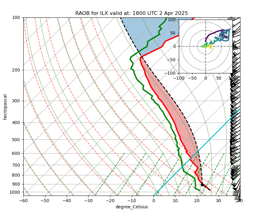
Now we are ready to create our skew-T. Plot it and save it as a PNG file.#
skew.ax.axvline , color must be singular.Additionally, some of the skew-T attributes (e.g. the shaded area between -12 and -18 C) may not be relevant (e.g., a warm-season convective case). Comment out those you don't wish to show.
# Create a new figure. The dimensions here give a good aspect ratio
fig = plt.figure(figsize=(9, 9))
skew = SkewT(fig, rotation=45)

# Plot the data using normal plotting functions, in this case using
# log scaling in Y, as dictated by the typical meteorological plot
skew.plot(P, T, 'r', linewidth=3)
skew.plot(P, Td, 'g', linewidth=3)
skew.plot_barbs(P[idx], u[idx], v[idx])
skew.ax.set_ylim(pBot, pTop)
skew.ax.set_xlim(tMin, tMax)

# Plot LCL as black dot
skew.plot(lclp, lclt, 'ko', markerfacecolor='black')

# Plot the parcel profile as a black line
skew.plot(P, parcel_prof, 'k', linestyle='--', linewidth=2)

# Shade areas of CAPE and CIN
skew.shade_cin(P, T, parcel_prof)
skew.shade_cape(P, T, parcel_prof)

# Shade areas between a certain temperature (in this case, the DGZ)
#skew.shade_area(P.m,-18,-12,color=['purple'])
# Plot a zero degree isotherm
skew.ax.axvline(0, color='c', linestyle='-', linewidth=2)

# Add the relevant special lines
skew.plot_dry_adiabats()
skew.plot_moist_adiabats(colors='#58a358', linestyle='-')
skew.plot_mixing_lines()

plt.title(f"RAOB for {station} valid at: {raob_timeTitle}")
# Create a hodograph
# Create an inset axes object that is 30% width and height of the
# figure and put it in the upper right hand corner.
ax_hod = inset_axes(skew.ax, '30%', '30%', loc=1)
h = Hodograph(ax_hod, component_range=100.)
h.add_grid(increment=30)
h.plot_colormapped(u, v, df['height'])
plt.savefig (f"{station}_{raob_timeStr}_skewt.png")
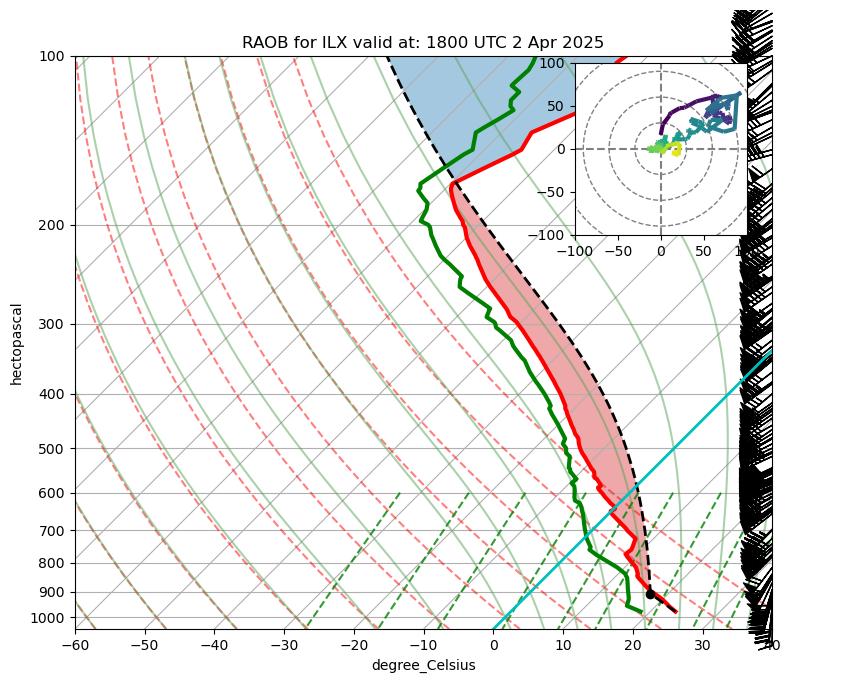
Here’s how the plot would appear if we hadn’t done the resampling. Note that the wind barbs are plotted at every level, and are harder to read:
# Create a new figure. The dimensions here give a good aspect ratio
fig = plt.figure(figsize=(9, 9))
skew = SkewT(fig, rotation=45)

# Plot the data using normal plotting functions, in this case using
# log scaling in Y, as dictated by the typical meteorological plot
skew.plot(P, T, 'r', linewidth=3)
skew.plot(P, Td, 'g', linewidth=3)
skew.plot_barbs(P, u, v)
skew.ax.set_ylim(pBot, pTop)
skew.ax.set_xlim(tMin, tMax)

# Plot LCL as black dot
skew.plot(lclp, lclt, 'ko', markerfacecolor='black')

# Plot the parcel profile as a black line
skew.plot(P, parcel_prof, 'k', linestyle='--', linewidth=2)

# Shade areas of CAPE and CIN
skew.shade_cin(P, T, parcel_prof)
skew.shade_cape(P, T, parcel_prof)

# Shade areas between a certain temperature (in this case, the DGZ)
#skew.shade_area(P.m,-18,-12,color=['purple'])
# Plot a zero degree isotherm
skew.ax.axvline(0, color='c', linestyle='-', linewidth=2)

# Add the relevant special lines
skew.plot_dry_adiabats()
skew.plot_moist_adiabats(colors='#58a358', linestyle='-')
skew.plot_mixing_lines()

plt.title(f"RAOB for {station} valid at: {raob_timeTitle}")

# Create a hodograph
# Create an inset axes object that is 30% width and height of the
# figure and put it in the upper right hand corner.
ax_hod = inset_axes(skew.ax, '30%', '30%', loc=1)
h = Hodograph(ax_hod, component_range=100.)
h.add_grid(increment=30)
h.plot_colormapped(u, v, df['height'])  # Plot a line colored by a parameter
<matplotlib.collections.LineCollection at 0x14825781fc80>
Here is a link to a map of NWS RAOB sites.
Depending on the situation, you may want to omit plotting the DGZ, LCL, parcel path, CAPE/CIN, freezing line, and/or move the location of the hodograph.