.ipynb .pdf

repository open issue suggest edit

Contents

Xarray 8: GRIB Data

Overview

1. Explore the differences between GRIB and NetCDF formats

2. Work with GRIB output from the HRRR regional model

3. Visualize data that is non-global in extent

Prerequisites

Concepts	Importance	Notes
Xarray Lessons 1-7	Necessary

• Time to learn: 30 minutes

---

Imports

import numpy as np
from datetime import datetime
import xarray as xr
import pandas as pd
import matplotlib.pyplot as plt
from matplotlib import colors
import cartopy.crs as ccrs
import cartopy.feature as cfeat
from metpy.plots import USCOUNTIES

GRIB vs NetCDF formats

Advantages of GRIB:

1. WMO-certifed format. Almost all NWP output that is generated by a national meteorological service will be in GRIB format.

2. Compresses well (GRIB version 2 only)

3. Still used for initial / boundary conditions in WRF.

4. “Well-behaved” GRIB data can be fairly easily translated into self-describing NetCDF format. A THREDDS server performs this translation on demand, thus presenting the user with data that looks to be in NetCDF format even if the actual data is in GRIB.

Disadvantages of GRIB:

1. Not self-describing (unlike NetCDF). A GRIB data file must be accompanied by a set of tables that decodes fields into their actual physicall-relevant names.

2. Despte being a WMO standard, there is no central source to maintain such tables. Often times, as new models get released, the existing tables that one might be using may not be updated with new parameters. Best strategy: update your GRIB software libraries often (and hope other things don’t break as a result).

3. As tables change, there is no guarantee that a GRIB file you read one year might decode the same way another year.

4. Grids are written out sequentially to an output GRIB file. As a result, performing temporal and especially spatial subsetting, such as we can do in Xarray with NetCDF or Zarr data, is very difficult.

Examine GRIB output from the HRRR regional model

We have downloaded a small subset of HRRR model output from the U. of Utah’s HRRR Archive and placed it in /spare11/atm533/data. The data consists of analysis and 1-6 hour forecast output from the 1600 UTC run of the HRRR on 7 October 2020; a period when eastern New York experienced a derecho-like event, very unusual for the time of year.

Specify the date and time; convert from datetime format to string.

date = datetime(2020,10,7,16)
date

datetime.datetime(2020, 10, 7, 16, 0)

YYYYMMDDHH = date.strftime('%Y%m%d%H')
YYYYMMDDHH

'2020100716'

Set forecast hour and convert to a string; pad string with a leading 0 if < 10 (see https://stackoverflow.com/questions/39402795/how-to-pad-a-string-with-leading-zeros-in-python-3/39402910)

fhr = 4
fhrStr = f'{fhr:02}'
fhrStr

'04'

Open the GRIB2 files containing forecasted composite reflectivity data. We use Xarray’s cfgrib engine to read in this type of data. There is also a file containing u- and v- components of the wind at 10 and 80 m above ground level.

refcFile = '/spare11/atm533/data/' + YYYYMMDDHH + '_hrrr_REFC.grib2'
windFile = '/spare11/atm533/data/' + YYYYMMDDHH + '_hrrr_WIND.grib2'

refcFile

'/spare11/atm533/data/2020100716_hrrr_REFC.grib2'

ds = xr.open_dataset(refcFile,engine='cfgrib')

This is another Xarray Dataset, consisting of data variables (one in this case), coordinate variables, dimensions and attributes. However, the dimension names and coordinate variables look different than in ERA-5.

ds

<xarray.Dataset>
Dimensions:     (step: 7, y: 1059, x: 1799)
Coordinates:
    time        datetime64[ns] ...
  * step        (step) timedelta64[ns] 00:00:00 01:00:00 ... 05:00:00 06:00:00
    atmosphere  float64 ...
    latitude    (y, x) float64 ...
    longitude   (y, x) float64 ...
    valid_time  (step) datetime64[ns] ...
Dimensions without coordinates: y, x
Data variables:
    refc        (step, y, x) float32 ...
Attributes:
    GRIB_edition:            2
    GRIB_centre:             kwbc
    GRIB_centreDescription:  US National Weather Service - NCEP
    GRIB_subCentre:          0
    Conventions:             CF-1.7
    institution:             US National Weather Service - NCEP
    history:                 2023-10-12T15:57 GRIB to CDM+CF via cfgrib-0.9.1...

xarray.Dataset

• Dimensions:
  • step: 7
  • y: 1059
  • x: 1799
• Coordinates: (6)
  • time
    ()
    datetime64[ns]
    ...

    long_name :

    initial time of forecast

    standard_name :

    forecast_reference_time

    [1 values with dtype=datetime64[ns]]

  • step
    (step)
    timedelta64[ns]
    00:00:00 01:00:00 ... 06:00:00

    long_name :

    time since forecast_reference_time

    standard_name :

    forecast_period

    array([             0,  3600000000000,  7200000000000, 10800000000000,
           14400000000000, 18000000000000, 21600000000000], dtype='timedelta64[ns]')

  • atmosphere
    ()
    float64
    ...

    long_name :

    original GRIB coordinate for key: level(atmosphere)

    units :

    1

    [1 values with dtype=float64]

  • latitude
    (y, x)
    float64
    ...

    units :

    degrees_north

    standard_name :

    latitude

    long_name :

    latitude

    [1905141 values with dtype=float64]

  • longitude
    (y, x)
    float64
    ...

    units :

    degrees_east

    standard_name :

    longitude

    long_name :

    longitude

    [1905141 values with dtype=float64]

  • valid_time
    (step)
    datetime64[ns]
    ...

    standard_name :

    time

    long_name :

    time

    [7 values with dtype=datetime64[ns]]

• Data variables: (1)
  • refc
    (step, y, x)
    float32
    ...

    GRIB_paramId :

    260390

    GRIB_dataType :

    fc

    GRIB_numberOfPoints :

    1905141

    GRIB_typeOfLevel :

    atmosphere

    GRIB_stepUnits :

    1

    GRIB_stepType :

    instant

    GRIB_gridType :

    lambert

    GRIB_DxInMetres :

    3000.0

    GRIB_DyInMetres :

    3000.0

    GRIB_LaDInDegrees :

    38.5

    GRIB_Latin1InDegrees :

    38.5

    GRIB_Latin2InDegrees :

    38.5

    GRIB_LoVInDegrees :

    262.5

    GRIB_NV :

    0

    GRIB_Nx :

    1799

    GRIB_Ny :

    1059

    GRIB_cfName :

    unknown

    GRIB_cfVarName :

    unknown

    GRIB_gridDefinitionDescription :

    Lambert Conformal can be secant or tangent, conical or bipolar

    GRIB_iScansNegatively :

    0

    GRIB_jPointsAreConsecutive :

    0

    GRIB_jScansPositively :

    1

    GRIB_latitudeOfFirstGridPointInDegrees :

    21.138123

    GRIB_latitudeOfSouthernPoleInDegrees :

    0.0

    GRIB_longitudeOfFirstGridPointInDegrees :

    237.280472

    GRIB_longitudeOfSouthernPoleInDegrees :

    0.0

    GRIB_missingValue :

    3.4028234663852886e+38

    GRIB_name :

    Maximum/Composite radar reflectivity

    GRIB_shortName :

    refc

    GRIB_units :

    dB

    long_name :

    Maximum/Composite radar reflectivity

    units :

    dB

    standard_name :

    unknown

    [13335987 values with dtype=float32]

• Indexes: (1)
  • step
    PandasIndex

    PandasIndex(TimedeltaIndex(['0 days 00:00:00', '0 days 01:00:00', '0 days 02:00:00',
                    '0 days 03:00:00', '0 days 04:00:00', '0 days 05:00:00',
                    '0 days 06:00:00'],
                   dtype='timedelta64[ns]', name='step', freq=None))

• Attributes: (7)

  GRIB_edition :

  2

  GRIB_centre :

  kwbc

  GRIB_centreDescription :

  US National Weather Service - NCEP

  GRIB_subCentre :

  0

  Conventions :

  CF-1.7

  institution :

  US National Weather Service - NCEP

  history :

  2023-10-12T15:57 GRIB to CDM+CF via cfgrib-0.9.10.4/ecCodes-2.31.0 with {"source": "../../../../../../../spare11/atm533/data/2020100716_hrrr_REFC.grib2", "filter_by_keys": {}, "encode_cf": ["parameter", "time", "geography", "vertical"]}

We can create an Xarray DataArray object pointing to composite reflectivity just as we could for any other Xarray Data variable.

refc = ds.refc

refc

<xarray.DataArray 'refc' (step: 7, y: 1059, x: 1799)>
[13335987 values with dtype=float32]
Coordinates:
    time        datetime64[ns] ...
  * step        (step) timedelta64[ns] 00:00:00 01:00:00 ... 05:00:00 06:00:00
    atmosphere  float64 ...
    latitude    (y, x) float64 ...
    longitude   (y, x) float64 ...
    valid_time  (step) datetime64[ns] ...
Dimensions without coordinates: y, x
Attributes: (12/33)
    GRIB_paramId:                             260390
    GRIB_dataType:                            fc
    GRIB_numberOfPoints:                      1905141
    GRIB_typeOfLevel:                         atmosphere
    GRIB_stepUnits:                           1
    GRIB_stepType:                            instant
    ...                                       ...
    GRIB_name:                                Maximum/Composite radar reflect...
    GRIB_shortName:                           refc
    GRIB_units:                               dB
    long_name:                                Maximum/Composite radar reflect...
    units:                                    dB
    standard_name:                            unknown

xarray.DataArray

'refc'

• step: 7
• y: 1059
• x: 1799

• ...

  [13335987 values with dtype=float32]

• Coordinates: (6)
  • time
    ()
    datetime64[ns]
    ...

    long_name :

    initial time of forecast

    standard_name :

    forecast_reference_time

    [1 values with dtype=datetime64[ns]]

  • step
    (step)
    timedelta64[ns]
    00:00:00 01:00:00 ... 06:00:00

    long_name :

    time since forecast_reference_time

    standard_name :

    forecast_period

    array([             0,  3600000000000,  7200000000000, 10800000000000,
           14400000000000, 18000000000000, 21600000000000], dtype='timedelta64[ns]')

  • atmosphere
    ()
    float64
    ...

    long_name :

    original GRIB coordinate for key: level(atmosphere)

    units :

    1

    [1 values with dtype=float64]

  • latitude
    (y, x)
    float64
    ...

    units :

    degrees_north

    standard_name :

    latitude

    long_name :

    latitude

    [1905141 values with dtype=float64]

  • longitude
    (y, x)
    float64
    ...

    units :

    degrees_east

    standard_name :

    longitude

    long_name :

    longitude

    [1905141 values with dtype=float64]

  • valid_time
    (step)
    datetime64[ns]
    ...

    standard_name :

    time

    long_name :

    time

    [7 values with dtype=datetime64[ns]]

• Indexes: (1)
  • step
    PandasIndex

    PandasIndex(TimedeltaIndex(['0 days 00:00:00', '0 days 01:00:00', '0 days 02:00:00',
                    '0 days 03:00:00', '0 days 04:00:00', '0 days 05:00:00',
                    '0 days 06:00:00'],
                   dtype='timedelta64[ns]', name='step', freq=None))

• Attributes: (33)

  GRIB_paramId :

  260390

  GRIB_dataType :

  fc

  GRIB_numberOfPoints :

  1905141

  GRIB_typeOfLevel :

  atmosphere

  GRIB_stepUnits :

  1

  GRIB_stepType :

  instant

  GRIB_gridType :

  lambert

  GRIB_DxInMetres :

  3000.0

  GRIB_DyInMetres :

  3000.0

  GRIB_LaDInDegrees :

  38.5

  GRIB_Latin1InDegrees :

  38.5

  GRIB_Latin2InDegrees :

  38.5

  GRIB_LoVInDegrees :

  262.5

  GRIB_NV :

  0

  GRIB_Nx :

  1799

  GRIB_Ny :

  1059

  GRIB_cfName :

  unknown

  GRIB_cfVarName :

  unknown

  GRIB_gridDefinitionDescription :

  Lambert Conformal can be secant or tangent, conical or bipolar

  GRIB_iScansNegatively :

  0

  GRIB_jPointsAreConsecutive :

  0

  GRIB_jScansPositively :

  1

  GRIB_latitudeOfFirstGridPointInDegrees :

  21.138123

  GRIB_latitudeOfSouthernPoleInDegrees :

  0.0

  GRIB_longitudeOfFirstGridPointInDegrees :

  237.280472

  GRIB_longitudeOfSouthernPoleInDegrees :

  0.0

  GRIB_missingValue :

  3.4028234663852886e+38

  GRIB_name :

  Maximum/Composite radar reflectivity

  GRIB_shortName :

  refc

  GRIB_units :

  dB

  long_name :

  Maximum/Composite radar reflectivity

  units :

  dB

  standard_name :

  unknown

Create a contour-fill plot of forecasted radar reflectivity

Our goal is produce a contour-fill plot of radar reflectivity, using colors that mimic similar NWS products. So first, create a colormap that includes RGB triplets in hex format, starting at 5 dBZ and going up to 75 dBZ.

Define a colormap to be used to contour the reflectivity values.

def radar_colormap():
    hrrr_reflectivity_colors = [
    "#00ecec", # 5
    "#01a0f6", # 10
    "#0000f6", # 15
    "#00ff00", # 20
    "#00c800", # 25
    "#009000", # 30
    "#ffff00", # 35
    "#e7c000", # 40
    "#ff9000", # 45
    "#ff0000", # 50
    "#d60000", # 55
    "#c00000", # 60
    "#ff00ff", # 65
    "#9955c9", # 70
    "#808080"  # 75
    ]
    cmap = colors.ListedColormap(hrrr_reflectivity_colors)
    return cmap

refl_range = np.arange(5,76,5) # defines our contour intervals
cmap= radar_colormap() # defines the color map that will accompany our filled contours and colorbar

Set areal extent for full (CONUS) region

latN = 52
latS = 20
lonW = -125
lonE = -60

Set the native projection from the Dataset’s attributes.

lat1 = refc.attrs['GRIB_LaDInDegrees']
lon1 = refc.attrs['GRIB_LoVInDegrees']
slat1 = refc.attrs['GRIB_Latin1InDegrees']
slat2 = refc.attrs['GRIB_Latin2InDegrees']

print(lat1,lon1,slat1,slat2)
proj_data = ccrs.LambertConformal(central_longitude=lon1,
                             central_latitude=lat1,
                             standard_parallels=[slat1,slat2])

38.5 262.5 38.5 38.5

Set areal extent and projection for the subset (NY) region.

latN_sub = 45.2
latS_sub = 40.2
lonW_sub = -80.0
lonE_sub = -71.5
cLat_sub = (latN_sub + latS_sub)/2.
cLon_sub = (lonW_sub + lonE_sub )/2.

proj_sub = ccrs.LambertConformal(central_longitude=cLon_sub,
                             central_latitude=cLat_sub,
                             standard_parallels=[cLat_sub])

Remind ourselves of the dimensions. They do not resemble what we’ve seen in the ERA-5 datasets: instead of time, longitude, and latitude, we have step, y, and x. We can look at each one of them.

refc.dims 

('step', 'y', 'x')

refc.step

<xarray.DataArray 'step' (step: 7)>
array([             0,  3600000000000,  7200000000000, 10800000000000,
       14400000000000, 18000000000000, 21600000000000], dtype='timedelta64[ns]')
Coordinates:
    time        datetime64[ns] ...
  * step        (step) timedelta64[ns] 00:00:00 01:00:00 ... 05:00:00 06:00:00
    atmosphere  float64 ...
    valid_time  (step) datetime64[ns] ...
Attributes:
    long_name:      time since forecast_reference_time
    standard_name:  forecast_period

xarray.DataArray

'step'

• step: 7

• 00:00:00 01:00:00 02:00:00 03:00:00 04:00:00 05:00:00 06:00:00

  array([             0,  3600000000000,  7200000000000, 10800000000000,
         14400000000000, 18000000000000, 21600000000000], dtype='timedelta64[ns]')

• Coordinates: (4)
  • time
    ()
    datetime64[ns]
    ...

    long_name :

    initial time of forecast

    standard_name :

    forecast_reference_time

    [1 values with dtype=datetime64[ns]]

  • step
    (step)
    timedelta64[ns]
    00:00:00 01:00:00 ... 06:00:00

    long_name :

    time since forecast_reference_time

    standard_name :

    forecast_period

    array([             0,  3600000000000,  7200000000000, 10800000000000,
           14400000000000, 18000000000000, 21600000000000], dtype='timedelta64[ns]')

  • atmosphere
    ()
    float64
    ...

    long_name :

    original GRIB coordinate for key: level(atmosphere)

    units :

    1

    [1 values with dtype=float64]

  • valid_time
    (step)
    datetime64[ns]
    ...

    standard_name :

    time

    long_name :

    time

    [7 values with dtype=datetime64[ns]]

• Indexes: (1)
  • step
    PandasIndex

    PandasIndex(TimedeltaIndex(['0 days 00:00:00', '0 days 01:00:00', '0 days 02:00:00',
                    '0 days 03:00:00', '0 days 04:00:00', '0 days 05:00:00',
                    '0 days 06:00:00'],
                   dtype='timedelta64[ns]', name='step', freq=None))

• Attributes: (2)

  long_name :

  time since forecast_reference_time

  standard_name :

  forecast_period

refc.y

<xarray.DataArray 'y' (y: 1059)>
array([   0,    1,    2, ..., 1056, 1057, 1058])
Coordinates:
    time        datetime64[ns] ...
    atmosphere  float64 ...
Dimensions without coordinates: y

xarray.DataArray

'y'

• y: 1059

• 0 1 2 3 4 5 6 7 8 9 ... 1050 1051 1052 1053 1054 1055 1056 1057 1058

  array([   0,    1,    2, ..., 1056, 1057, 1058])

• Coordinates: (2)
  • time
    ()
    datetime64[ns]
    ...

    long_name :

    initial time of forecast

    standard_name :

    forecast_reference_time

    [1 values with dtype=datetime64[ns]]

  • atmosphere
    ()
    float64
    ...

    long_name :

    original GRIB coordinate for key: level(atmosphere)

    units :

    1

    [1 values with dtype=float64]

• Indexes: (0)
• Attributes: (0)

refc.x

<xarray.DataArray 'x' (x: 1799)>
array([   0,    1,    2, ..., 1796, 1797, 1798])
Coordinates:
    time        datetime64[ns] ...
    atmosphere  float64 ...
Dimensions without coordinates: x

xarray.DataArray

'x'

• x: 1799

• 0 1 2 3 4 5 6 7 8 9 ... 1790 1791 1792 1793 1794 1795 1796 1797 1798

  array([   0,    1,    2, ..., 1796, 1797, 1798])

• Coordinates: (2)
  • time
    ()
    datetime64[ns]
    ...

    long_name :

    initial time of forecast

    standard_name :

    forecast_reference_time

    [1 values with dtype=datetime64[ns]]

  • atmosphere
    ()
    float64
    ...

    long_name :

    original GRIB coordinate for key: level(atmosphere)

    units :

    1

    [1 values with dtype=float64]

• Indexes: (0)
• Attributes: (0)

We can see that these dimensions are just sequential index values for x and y, while the time steps are one hour at a time, expressed in nanoseconds. This makes it more difficult for us to use Xarray’s handy way of using dimension names for, among other things, selection and subsetting. Instead, we have to use a more NumPy/Pandas-way of using index numbers.

Here, we will pick one of the seven discrete times to display radar imagery. Let’s choose index 4 … valid at 2000 UTC 7 October … just as the squall line was impacting the Greater Capital District.

Select timestep index. Use it to not only plot the correct reflectivity array, but also to determine the date and time for the purposes of labeling. Note the three-step process:

idx = 4

1. Get the time as a NumPy Datetime64 object:

validTime = refc.valid_time[idx].values

validTime

numpy.datetime64('2020-10-07T20:00:00.000000000')

2. Convert into a Pandas Timestamp object:

validTime = pd.Timestamp(validTime) # Converts validTime to a Pandas Timestamp object

validTime

Timestamp('2020-10-07 20:00:00')

3. Use the datetime library’s strftime method to create a time string object:

timeStr = validTime.strftime("%Y-%m-%d %H%M UTC") # We can now use Datetime's strftime method to create a time string.

timeStr

'2020-10-07 2000 UTC'

Make the map

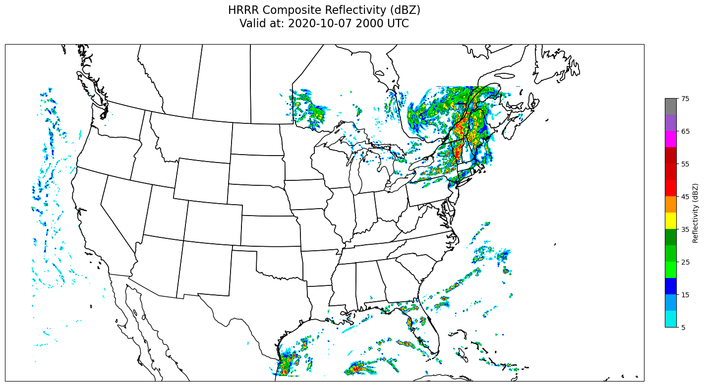
tl1 = "HRRR Composite Reflectivity (dBZ)"
tl2 = str('Valid at: '+ timeStr)
title_line = (tl1 + '\n' + tl2 + '\n')

First draw a radar map that covers the entire domain of the HRRR.

Warning: The HRRR stands for High Resolution Rapid Refresh. The horizontal dimensions are 1059 x 1799 ... approximately 3 km between gridpoints. As a result, the maps will take longer to render.

Tip: Omitting some of the cartographic features, especially the filled ones like *ocean*, *land*, and *lakes*, will speed things up.

res = '50m'
fig = plt.figure(figsize=(18,12))
ax = plt.subplot(1,1,1,projection=proj_data)
ax.set_extent((lonW,lonE,latS,latN))
#ax.add_feature (cfeat.LAND.with_scale(res))
#ax.add_feature (cfeat.OCEAN.with_scale(res))
ax.add_feature(cfeat.COASTLINE.with_scale(res))
#ax.add_feature (cfeat.LAKES.with_scale(res), alpha = 0.5)
ax.add_feature (cfeat.STATES.with_scale(res))
# don't include county lines here
#ax.add_feature(USCOUNTIES,edgecolor='grey', linewidth=1, zorder = 3 );
CF = ax.contourf(refc.longitude,refc.latitude,refc[idx],levels=refl_range,cmap=cmap,transform=ccrs.PlateCarree())
cbar = plt.colorbar(CF,fraction=0.046, pad=0.03,shrink=0.5)
cbar.ax.tick_params(labelsize=10)
cbar.ax.set_ylabel("Reflectivity (dBZ)",fontsize=10)
title = ax.set_title(title_line,fontsize=16)

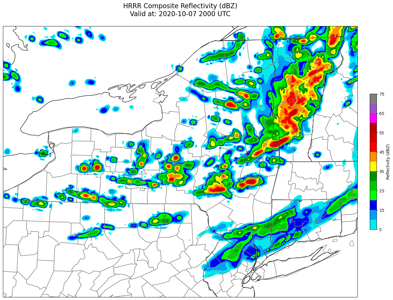
Now, plot the map over NYS.

res = '50m'
fig = plt.figure(figsize=(18,12))
ax = plt.subplot(1,1,1,projection=proj_sub)
ax.set_extent((lonW_sub,lonE_sub,latS_sub,latN_sub),crs=ccrs.PlateCarree())
#ax.add_feature (cfeat.LAND.with_scale(res))
#ax.add_feature (cfeat.OCEAN.with_scale(res))
ax.add_feature(cfeat.COASTLINE.with_scale(res))
#ax.add_feature (cfeat.LAKES.with_scale(res), alpha = 0.5)
ax.add_feature (cfeat.STATES.with_scale(res))
ax.add_feature(USCOUNTIES,edgecolor='grey', linewidth=1 );
CF = ax.contourf(refc.longitude,refc.latitude,refc[idx],levels=refl_range,cmap=cmap,transform=ccrs.PlateCarree())
cbar = plt.colorbar(CF,fraction=0.046, pad=0.03,shrink=0.5)
cbar.ax.tick_params(labelsize=10)
cbar.ax.set_ylabel("Reflectivity (dBZ)",fontsize=10)
title = ax.set_title(title_line,fontsize=16)

To think about:
1. How would you plot different times? Is there just a single cell whose value needs to be change?
2. What if you wanted to loop over all seven times? Why does a Jupyter notebook make it a bit more difficult to do this?
3. Try loading and plotting the WIND Dataset. It consists of u- and v- components of wind at 10 and 80 m. Can you use the same call to xarray.open_dataset that you did for reflectivity?

---

Summary

• Using Xarray’s cfgrib data engine, we can analyze and display data in GRIB format.

• In general, GRIB data is “messier” than data in a self-describing format, such as NetCDF.

What’s Next?

In the next notebook, we’ll explore HRRR data that is stored “in the cloud”, in a format called Zarr.

Resources and References

1. GRIB Reference

2. MetPy Monday Episode 135: Reading GRIB

3. MetPy Monday Episode 136: Delving into unknown NDFD GRIB data

4. MetPy Monday Episode 137: Finding GRIB forecast times and attaching units