Pandas 4: Working with date- and time-based data
Contents
Pandas 4: Working with date- and time-based data

Overview
In this notebook, we’ll work with Pandas DataFrame and Series objects to do the following:
Work with Pandas’ implementation of methods and attributes from Python’s
datetimelibraryRelabel a Series from a column whose values are date and time strings
Employ a
lambdafunction to convert date/time strings todatetimeobjectsUse Pandas’ built-in
plotfunction to generate a basic time series plotImprove the look of the time series plot by using Matplotlib
We’ll once again use NYS Mesonet data, but for the entire day of 2 September 2021.
Prerequisites
Concepts |
Importance |
Notes |
|---|---|---|
Matplotlib |
Necessary |
|
Datetime |
Helpful |
|
Pandas |
Necessary |
Notebooks 1-3 |
Time to learn: 30 minutes
Imports
import pandas as pd
import matplotlib.pyplot as plt
from datetime import datetime
Create a DataFrame objects from a csv file that contains NYSM observational data. Choose the station ID as the row index.
dataFile = '/spare11/atm533/data/nysm_data_20210902.csv'
nysm_data = pd.read_csv(dataFile,index_col='station')
Examine the nysm_data object.
nysm_data
| time | temp_2m [degC] | temp_9m [degC] | relative_humidity [percent] | precip_incremental [mm] | precip_local [mm] | precip_max_intensity [mm/min] | avg_wind_speed_prop [m/s] | max_wind_speed_prop [m/s] | wind_speed_stddev_prop [m/s] | ... | snow_depth [cm] | frozen_soil_05cm [bit] | frozen_soil_25cm [bit] | frozen_soil_50cm [bit] | soil_temp_05cm [degC] | soil_temp_25cm [degC] | soil_temp_50cm [degC] | soil_moisture_05cm [m^3/m^3] | soil_moisture_25cm [m^3/m^3] | soil_moisture_50cm [m^3/m^3] | |
|---|---|---|---|---|---|---|---|---|---|---|---|---|---|---|---|---|---|---|---|---|---|
| station | |||||||||||||||||||||
| ADDI | 2021-09-02 00:00:00 UTC | 14.8 | 14.8 | 93.1 | 0.0 | 9.56 | 0.0 | 3.0 | 6.0 | 1.1 | ... | NaN | 0.0 | 0.0 | 0.0 | 20.1 | 20.5 | 19.9 | 0.51 | 0.44 | 0.44 |
| ADDI | 2021-09-02 00:05:00 UTC | 14.6 | 14.7 | 93.3 | 0.0 | 0.00 | 0.0 | 2.8 | 4.2 | 0.6 | ... | NaN | 0.0 | 0.0 | 0.0 | 20.1 | 20.5 | 19.9 | 0.51 | 0.44 | 0.44 |
| ADDI | 2021-09-02 00:10:00 UTC | 14.6 | 14.6 | 93.6 | 0.0 | 0.00 | 0.0 | 3.0 | 4.9 | 0.9 | ... | NaN | 0.0 | 0.0 | 0.0 | 20.1 | 20.5 | 19.9 | 0.51 | 0.44 | 0.44 |
| ADDI | 2021-09-02 00:15:00 UTC | 14.6 | 14.6 | 93.7 | 0.0 | 0.00 | 0.0 | 2.9 | 5.3 | 0.9 | ... | NaN | 0.0 | 0.0 | 0.0 | 20.1 | 20.5 | 19.9 | 0.51 | 0.44 | 0.44 |
| ADDI | 2021-09-02 00:20:00 UTC | 14.5 | 14.5 | 93.9 | 0.0 | 0.00 | 0.0 | 2.5 | 4.5 | 0.7 | ... | NaN | 0.0 | 0.0 | 0.0 | 20.1 | 20.5 | 19.9 | 0.51 | 0.44 | 0.44 |
| ... | ... | ... | ... | ... | ... | ... | ... | ... | ... | ... | ... | ... | ... | ... | ... | ... | ... | ... | ... | ... | ... |
| YORK | 2021-09-02 23:35:00 UTC | 15.9 | 16.3 | 69.8 | 0.0 | 0.21 | 0.0 | 2.2 | 4.0 | 0.6 | ... | NaN | 0.0 | 0.0 | 0.0 | 20.5 | 20.8 | 21.1 | 0.12 | 0.24 | 0.23 |
| YORK | 2021-09-02 23:40:00 UTC | 15.9 | 16.2 | 70.2 | 0.0 | 0.21 | 0.0 | 2.2 | 3.4 | 0.5 | ... | NaN | 0.0 | 0.0 | 0.0 | 20.5 | 20.9 | 21.1 | 0.12 | 0.24 | 0.23 |
| YORK | 2021-09-02 23:45:00 UTC | 15.6 | 16.0 | 71.6 | 0.0 | 0.21 | 0.0 | 1.6 | 3.1 | 0.4 | ... | NaN | 0.0 | 0.0 | 0.0 | 20.5 | 20.7 | 21.1 | 0.12 | 0.24 | 0.23 |
| YORK | 2021-09-02 23:50:00 UTC | 15.5 | 16.0 | 72.1 | 0.0 | 0.21 | 0.0 | 2.2 | 2.9 | 0.4 | ... | NaN | 0.0 | 0.0 | 0.0 | 20.5 | 20.8 | 21.1 | 0.12 | 0.24 | 0.24 |
| YORK | 2021-09-02 23:55:00 UTC | 15.1 | 15.7 | 73.7 | 0.0 | 0.21 | 0.0 | 1.5 | 2.3 | 0.4 | ... | NaN | 0.0 | 0.0 | 0.0 | 20.5 | 20.9 | 21.1 | 0.12 | 0.24 | 0.23 |
36288 rows × 29 columns
Work with Pandas’ implementation of methods and attributes from Python’s datetime library
Relabel a Series from a column whose values are date and time strings
First, let’s load 5-minute accumulated precipitation for the Manhattan site.
# Select the column and row of interest
prcpMANH = nysm_data['precip_incremental [mm]'].loc['MANH']
prcpMANH
station
MANH    0.53
MANH    1.37
MANH    4.37
MANH    1.83
MANH    2.00
        ...
MANH    0.00
MANH    0.00
MANH    0.00
MANH    0.00
MANH    0.00
Name: precip_incremental [mm], Length: 288, dtype: float64
Next, let’s inspect the column correpsonding to date and time from the DataFrame.
timeSer = nysm_data['time']
timeSer
station
ADDI    2021-09-02 00:00:00 UTC
ADDI    2021-09-02 00:05:00 UTC
ADDI    2021-09-02 00:10:00 UTC
ADDI    2021-09-02 00:15:00 UTC
ADDI    2021-09-02 00:20:00 UTC
                 ...
YORK    2021-09-02 23:35:00 UTC
YORK    2021-09-02 23:40:00 UTC
YORK    2021-09-02 23:45:00 UTC
YORK    2021-09-02 23:50:00 UTC
YORK    2021-09-02 23:55:00 UTC
Name: time, Length: 36288, dtype: object
The dtype: object signifies that the values for time are being treated as a string. When working with time-based arrays, we want to treat them differently than a generic string type … instead, let’s treat them as datetime objects (derived from NumPy: see reference at end of notebook).
First, let’s look at the output after converting the Series from string to datetime. To do that, we’ll use the to_datetime method in Pandas. We pass in the Series, which consists of an array of strings, and then specify how the strings are formatted. See the reference at the end of the notebook for a guide to formatting date/time strings.
pd.to_datetime(timeSer, format = "%Y-%m-%d %H:%M:%S UTC", utc=True)
station
ADDI   2021-09-02 00:00:00+00:00
ADDI   2021-09-02 00:05:00+00:00
ADDI   2021-09-02 00:10:00+00:00
ADDI   2021-09-02 00:15:00+00:00
ADDI   2021-09-02 00:20:00+00:00
                  ...
YORK   2021-09-02 23:35:00+00:00
YORK   2021-09-02 23:40:00+00:00
YORK   2021-09-02 23:45:00+00:00
YORK   2021-09-02 23:50:00+00:00
YORK   2021-09-02 23:55:00+00:00
Name: time, Length: 36288, dtype: datetime64[ns, UTC]
Notice that the dtype of the Series has changed to datetime64, with precision to the nanosecond level and a timezone of UTC.
With the use of a lambda function, we can accomplish the string–>datetime conversion directly in the call to read_csv. We’ll also now set the row index to be time.
# First define the format and then define the function
format = "%Y-%m-%d %H:%M:%S UTC"
# This function will iterate over each string in a 1-d array
# and use Pandas' implementation of strptime to convert the string into a datetime object.
parseTime = lambda x: datetime.strptime(x, format)
Remind ourselves of how Pandas’ read_csv method works:
pd.read_csv?
Re-create the nysm_data DataFrame, with appropriate additional arguments to read_csv (including our lambda function, via the date_parser argument)
nysm_data = pd.read_csv(dataFile,index_col=1,parse_dates=['time'], date_parser=parseTime)
nysm_data.head(2)
| station | temp_2m [degC] | temp_9m [degC] | relative_humidity [percent] | precip_incremental [mm] | precip_local [mm] | precip_max_intensity [mm/min] | avg_wind_speed_prop [m/s] | max_wind_speed_prop [m/s] | wind_speed_stddev_prop [m/s] | ... | snow_depth [cm] | frozen_soil_05cm [bit] | frozen_soil_25cm [bit] | frozen_soil_50cm [bit] | soil_temp_05cm [degC] | soil_temp_25cm [degC] | soil_temp_50cm [degC] | soil_moisture_05cm [m^3/m^3] | soil_moisture_25cm [m^3/m^3] | soil_moisture_50cm [m^3/m^3] | |
|---|---|---|---|---|---|---|---|---|---|---|---|---|---|---|---|---|---|---|---|---|---|
| time | |||||||||||||||||||||
| 2021-09-02 00:00:00 | ADDI | 14.8 | 14.8 | 93.1 | 0.0 | 9.56 | 0.0 | 3.0 | 6.0 | 1.1 | ... | NaN | 0.0 | 0.0 | 0.0 | 20.1 | 20.5 | 19.9 | 0.51 | 0.44 | 0.44 |
| 2021-09-02 00:05:00 | ADDI | 14.6 | 14.7 | 93.3 | 0.0 | 0.00 | 0.0 | 2.8 | 4.2 | 0.6 | ... | NaN | 0.0 | 0.0 | 0.0 | 20.1 | 20.5 | 19.9 | 0.51 | 0.44 | 0.44 |
2 rows × 29 columns
Now time is the DataFrame’s row index. Let’s inspect this index; it’s much like a generic Pandas RangeIndex, but specific for date/time purposes:
timeIndx = nysm_data.index
timeIndx
DatetimeIndex(['2021-09-02 00:00:00', '2021-09-02 00:05:00',
               '2021-09-02 00:10:00', '2021-09-02 00:15:00',
               '2021-09-02 00:20:00', '2021-09-02 00:25:00',
               '2021-09-02 00:30:00', '2021-09-02 00:35:00',
               '2021-09-02 00:40:00', '2021-09-02 00:45:00',
               ...
               '2021-09-02 23:10:00', '2021-09-02 23:15:00',
               '2021-09-02 23:20:00', '2021-09-02 23:25:00',
               '2021-09-02 23:30:00', '2021-09-02 23:35:00',
               '2021-09-02 23:40:00', '2021-09-02 23:45:00',
               '2021-09-02 23:50:00', '2021-09-02 23:55:00'],
              dtype='datetime64[ns]', name='time', length=36288, freq=None)
Note that the timezone is missing. The read_csv method does not provide a means to specify the timezone. We can take care of that though with the tz_localize method.
timeIndx = timeIndx.tz_localize(tz='UTC')
timeIndx
DatetimeIndex(['2021-09-02 00:00:00+00:00', '2021-09-02 00:05:00+00:00',
               '2021-09-02 00:10:00+00:00', '2021-09-02 00:15:00+00:00',
               '2021-09-02 00:20:00+00:00', '2021-09-02 00:25:00+00:00',
               '2021-09-02 00:30:00+00:00', '2021-09-02 00:35:00+00:00',
               '2021-09-02 00:40:00+00:00', '2021-09-02 00:45:00+00:00',
               ...
               '2021-09-02 23:10:00+00:00', '2021-09-02 23:15:00+00:00',
               '2021-09-02 23:20:00+00:00', '2021-09-02 23:25:00+00:00',
               '2021-09-02 23:30:00+00:00', '2021-09-02 23:35:00+00:00',
               '2021-09-02 23:40:00+00:00', '2021-09-02 23:45:00+00:00',
               '2021-09-02 23:50:00+00:00', '2021-09-02 23:55:00+00:00'],
              dtype='datetime64[ns, UTC]', name='time', length=36288, freq=None)
If this were a Series, not an index, use this Series-specific method instead:
timeIndx= timeIndx.dt.tz_localize(tz='UTC')
Since it’s a datetime object now, we can apply all sorts of time/date operations to it. For example, let’s convert to Eastern time.
timeIndx = timeIndx.tz_convert(tz='US/Eastern')
timeIndx
DatetimeIndex(['2021-09-01 20:00:00-04:00', '2021-09-01 20:05:00-04:00',
               '2021-09-01 20:10:00-04:00', '2021-09-01 20:15:00-04:00',
               '2021-09-01 20:20:00-04:00', '2021-09-01 20:25:00-04:00',
               '2021-09-01 20:30:00-04:00', '2021-09-01 20:35:00-04:00',
               '2021-09-01 20:40:00-04:00', '2021-09-01 20:45:00-04:00',
               ...
               '2021-09-02 19:10:00-04:00', '2021-09-02 19:15:00-04:00',
               '2021-09-02 19:20:00-04:00', '2021-09-02 19:25:00-04:00',
               '2021-09-02 19:30:00-04:00', '2021-09-02 19:35:00-04:00',
               '2021-09-02 19:40:00-04:00', '2021-09-02 19:45:00-04:00',
               '2021-09-02 19:50:00-04:00', '2021-09-02 19:55:00-04:00'],
              dtype='datetime64[ns, US/Eastern]', name='time', length=36288, freq=None)
(Yes, it automatically accounts for Standard or Daylight time!)
Use Pandas’ built-in plot function … which leverages Matplotlib:
Select all the rows for site MANH
condition = nysm_data['station'] == 'MANH'
MANH = nysm_data.loc[condition]
Generate a basic time series plot by passing the desired column to Pandas’ plot method:
prcp = MANH['precip_incremental [mm]']
prcp.plot()
<AxesSubplot:xlabel='time'>
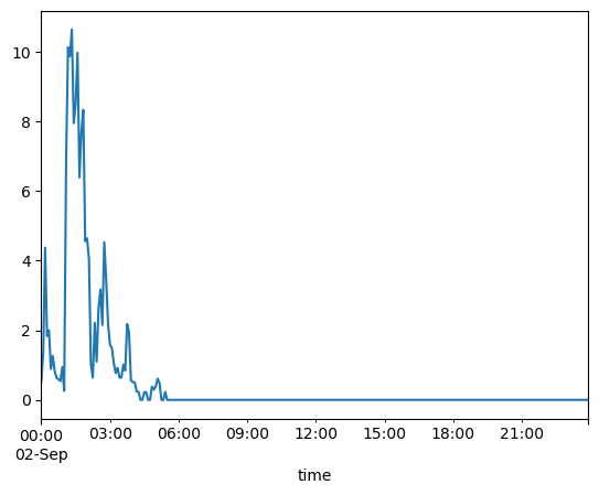
That was a way to get a quick look at the data and verify it looks reasonable. Now, let’s pretty it up by using Matplotlib functions.
We’ll draw a line plot, passing in time and wind gust speed for the x- and y-axes, respectively. Follow the same procedure as we did in the Matplotlib notebooks from week 3.
plt.style.use("seaborn")
fig = plt.figure(figsize=(11,8.5))
ax = fig.add_subplot(1,1,1)
ax.set_xlabel ('Date and Time')
ax.set_ylabel ('5-min accum. precip (mm)')
ax.set_title ("Manhattan, NY 5-minute accumulated precip associated with the remnants of Hurricane Ida")
ax.plot (timeIndx, prcp)
---------------------------------------------------------------------------
ValueError                                Traceback (most recent call last)
Input In [17], in <cell line: 7>()
      5 ax.set_ylabel ('5-min accum. precip (mm)')
      6 ax.set_title ("Manhattan, NY 5-minute accumulated precip associated with the remnants of Hurricane Ida")
----> 7 ax.plot (timeIndx, prcp)

File /knight/anaconda_aug22/envs/aug22_env/lib/python3.10/site-packages/matplotlib/axes/_axes.py:1635, in Axes.plot(self, scalex, scaley, data, *args, **kwargs)
   1393 """
   1394 Plot y versus x as lines and/or markers.
   1395
   (...)
   1632 (``'green'``) or hex strings (``'#008000'``).
   1633 """
   1634 kwargs = cbook.normalize_kwargs(kwargs, mlines.Line2D)
-> 1635 lines = [*self._get_lines(*args, data=data, **kwargs)]
   1636 for line in lines:
   1637     self.add_line(line)

File /knight/anaconda_aug22/envs/aug22_env/lib/python3.10/site-packages/matplotlib/axes/_base.py:312, in _process_plot_var_args.__call__(self, data, *args, **kwargs)
    310     this += args[0],
    311     args = args[1:]
--> 312 yield from self._plot_args(this, kwargs)

File /knight/anaconda_aug22/envs/aug22_env/lib/python3.10/site-packages/matplotlib/axes/_base.py:498, in _process_plot_var_args._plot_args(self, tup, kwargs, return_kwargs)
    495     self.axes.yaxis.update_units(y)
    497 if x.shape[0] != y.shape[0]:
--> 498     raise ValueError(f"x and y must have same first dimension, but "
    499                      f"have shapes {x.shape} and {y.shape}")
    500 if x.ndim > 2 or y.ndim > 2:
    501     raise ValueError(f"x and y can be no greater than 2D, but have "
    502                      f"shapes {x.shape} and {y.shape}")

ValueError: x and y must have same first dimension, but have shapes (36288,) and (288,)
Didn’t work!!! Look at the error message above!
This is a mismatch between array sizes. The time index is based on the entire Dataframe, which has 12 x 24 x 126 rows, while the Manhattan precip array is only 12 x 24!
Let’s set a condition where we match only those times that are in the same row as the Manhattan station id.
condition = nysm_data['station'] == 'MANH'
timeIndxMANH = timeIndx[condition]
timeIndxMANH
DatetimeIndex(['2021-09-01 20:00:00-04:00', '2021-09-01 20:05:00-04:00',
               '2021-09-01 20:10:00-04:00', '2021-09-01 20:15:00-04:00',
               '2021-09-01 20:20:00-04:00', '2021-09-01 20:25:00-04:00',
               '2021-09-01 20:30:00-04:00', '2021-09-01 20:35:00-04:00',
               '2021-09-01 20:40:00-04:00', '2021-09-01 20:45:00-04:00',
               ...
               '2021-09-02 19:10:00-04:00', '2021-09-02 19:15:00-04:00',
               '2021-09-02 19:20:00-04:00', '2021-09-02 19:25:00-04:00',
               '2021-09-02 19:30:00-04:00', '2021-09-02 19:35:00-04:00',
               '2021-09-02 19:40:00-04:00', '2021-09-02 19:45:00-04:00',
               '2021-09-02 19:50:00-04:00', '2021-09-02 19:55:00-04:00'],
              dtype='datetime64[ns, US/Eastern]', name='time', length=288, freq=None)
plt.style.use("seaborn")
fig = plt.figure(figsize=(11,8.5))
ax = fig.add_subplot(1,1,1)
ax.set_xlabel ('Date and Time')
ax.set_ylabel ('5-min accum. precip (mm)')
ax.set_title ("Manhattan, NY 5-minute accumulated precip associated with the remnants of Hurricane Ida")
ax.plot (timeIndxMANH, prcp);
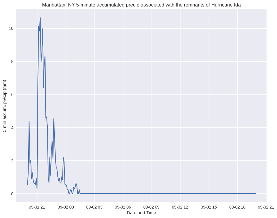
That’s looking better! We still have work to do to improve the labeling of the x-axis tick marks, but we’ll save that for another time.
Summary
Use a
lambdafunction to convert Date/time strings into PythondatetimeobjectsPandas’
plotmethod allows for a quick visualization ofDataFrameandSeriesobjects.x- and y- arrays must be of the same size in order to be plotted.
What’s Next?
Coming up next week, we will conclude our exploration of Pandas.