Pandas 2: NYS Mesonet Map
Contents

Pandas 2: NYS Mesonet Map
Overview
In this notebook, we’ll use Cartopy, Matplotlib, and Pandas (with a little help from MetPy) to read in, manipulate, and visualize data from the New York State Mesonet.
We’ll focus on a particular time on the evening of 1 September 2021, when the remnants of Hurricane Ida were impacting the greater New York City region.
Prerequisites
Concepts |
Importance |
Notes |
|---|---|---|
Matplotlib |
Necessary |
|
Cartopy |
Necessary |
|
Pandas |
Necessary |
Intro |
MetPy |
Helpful |
Time to learn: 30 minutes
Imports
import matplotlib.pyplot as plt
import numpy as np
import pandas as pd
from cartopy import crs as ccrs
from cartopy import feature as cfeature
from metpy.calc import wind_components
from metpy.units import units
from metpy.plots import StationPlot
ERROR 1: PROJ: proj_create_from_database: Open of /knight/anaconda_aug22/envs/aug22_env/share/proj failed
Create Pandas DataFrame objects based on two csv files; one contains the site locations, while the other contains the hourly data.
nysm_sites = pd.read_csv('/spare11/atm533/data/nysm_sites.csv')
nysm_data = pd.read_csv('/spare11/atm533/data/nysm_data_2021090202.csv')
Create Series objects for several columns from the two DataFrames.
First, remind ourselves of the column names for these two DataFrames.
nysm_sites.columns
Index(['stid', 'number', 'name', 'lat', 'lon', 'elevation', 'county',
       'nearest_city', 'state', 'distance_from_town [km]',
       'direction_from_town [degrees]', 'climate_division',
       'climate_division_name', 'wfo', 'commissioned', 'decommissioned'],
      dtype='object')
nysm_data.columns
Index(['station', 'time', 'temp_2m [degC]', 'temp_9m [degC]',
       'relative_humidity [percent]', 'precip_incremental [mm]',
       'precip_local [mm]', 'precip_max_intensity [mm/min]',
       'avg_wind_speed_prop [m/s]', 'max_wind_speed_prop [m/s]',
       'wind_speed_stddev_prop [m/s]', 'wind_direction_prop [degrees]',
       'wind_direction_stddev_prop [degrees]', 'avg_wind_speed_sonic [m/s]',
       'max_wind_speed_sonic [m/s]', 'wind_speed_stddev_sonic [m/s]',
       'wind_direction_sonic [degrees]',
       'wind_direction_stddev_sonic [degrees]', 'solar_insolation [W/m^2]',
       'station_pressure [mbar]', 'snow_depth [cm]', 'frozen_soil_05cm [bit]',
       'frozen_soil_25cm [bit]', 'frozen_soil_50cm [bit]',
       'soil_temp_05cm [degC]', 'soil_temp_25cm [degC]',
       'soil_temp_50cm [degC]', 'soil_moisture_05cm [m^3/m^3]',
       'soil_moisture_25cm [m^3/m^3]', 'soil_moisture_50cm [m^3/m^3]'],
      dtype='object')
Create several Series objects for particular columns of interest. Pay attention to which DataFrame provides the particular Series!
stid = nysm_sites['stid']
lats = nysm_sites['lat']
lons = nysm_sites['lon']

time = nysm_data['time']
tmpc = nysm_data['temp_2m [degC]']
rh   = nysm_data['relative_humidity [percent]']
pres = nysm_data['station_pressure [mbar]']
wspd = nysm_data['max_wind_speed_prop [m/s]']
drct = nysm_data['wind_direction_prop [degrees]']
pinc = nysm_data['precip_incremental [mm]']
ptot = nysm_data['precip_local [mm]']
pint = nysm_data['precip_max_intensity [mm/min]']
Examine one or more of these Series.
tmpc
0      13.3
1      14.0
2      14.8
3      16.0
4      14.3
       ...
121    12.9
122    13.8
123    15.7
124    14.0
125    12.0
Name: temp_2m [degC], Length: 126, dtype: float64
Series object.# Write your code below
Series objects contain data stored as NumPy arrays. As a result, we can take advantage of broadcasting to perform operations on all array elements without needing to construct a Python for loop. Convert the temperature and wind speed arrays to Fahrenheit and knots, respectively.
tmpf = tmpc * 1.8 + 32
wspk = wspd * 1.94384
Examine the new Series. Note that every element of the array has been calculated using the arithemtic above … in just one line of code per Series!
tmpf
0      55.94
1      57.20
2      58.64
3      60.80
4      57.74
       ...
121    55.22
122    56.84
123    60.26
124    57.20
125    53.60
Name: temp_2m [degC], Length: 126, dtype: float64
Series' name attribute:tmpf.name = 'temp_2m [degF]'
tmpf
0      55.94
1      57.20
2      58.64
3      60.80
4      57.74
       ...
121    55.22
122    56.84
123    60.26
124    57.20
125    53.60
Name: temp_2m [degF], Length: 126, dtype: float64
Next, use another statistical method available to Series: in this case, the maximum value among all elements of the array.
wspk.max()
32.07336
Our goal is to make a map of NYSM observations, which includes the wind velocity. The convention is to plot wind velocity using wind barbs. The MetPy library allows us to not only make such a map, but perform a variety of meteorologically-relevant calculations and diagnostics. Here, we will use such a calculation, which will determine the two scalar components of wind velocity (u and v), from wind speed and direction. We will use MetPy’s wind_components method.
This method requires us to do the following:
Extract the Numpy arrays from the windspeed and direction
Seriesobjects via thevaluesattributeAttach units to these arrays using MetPy’s
unitsclass
We can accomplish everything in this single line of code:
u, v = wind_components(wspk.values * units.knots, drct.values * units.degree)
Take a look at one of the output components:
u
| Magnitude | [3.1076105228416284 0.3525481021992311 3.4248560097185075 |
|---|---|
| Units | knot |
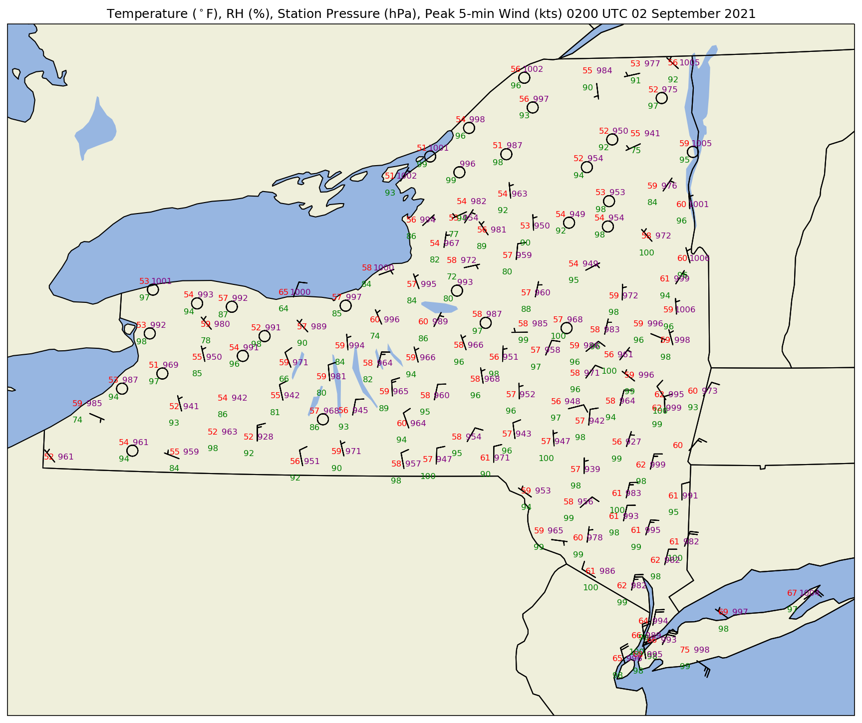
Now, let’s plot several of the meteorological values on a map. We will use Matplotlib and Cartopy, as well as MetPy’s StationPlot method.
Plot the map, centered over NYS, with add some geographic features, and the mesonet data.
For a meteorological surface station plot, let’s take advantage of the Metpy package, and its StationPlot method.
Be patient: this may take a minute or so to plot, if you chose the highest resolution for the shapefiles!
# Set the domain for defining the plot region.
latN = 45.2
latS = 40.2
lonW = -80.0
lonE = -72.0
cLat = (latN + latS)/2
cLon = (lonW + lonE )/2

res = '50m'
proj = ccrs.LambertConformal(central_longitude=cLon, central_latitude=cLat)

fig = plt.figure(figsize=(18,12),dpi=150) # Increase the dots per inch from default 100 to make plot easier to read
ax = fig.add_subplot(1,1,1,projection=proj)
ax.set_extent ([lonW,lonE,latS,latN])
ax.add_feature (cfeature.LAND.with_scale(res))
ax.add_feature (cfeature.OCEAN.with_scale(res))
ax.add_feature(cfeature.COASTLINE.with_scale(res))
ax.add_feature (cfeature.LAKES.with_scale(res))
ax.add_feature (cfeature.STATES.with_scale(res));

# Create a station plot pointing to an Axes to draw on as well as the location of points
stationplot = StationPlot(ax, lons, lats, transform=ccrs.PlateCarree(),
                          fontsize=8)

stationplot.plot_parameter('NW', tmpf, color='red')
stationplot.plot_parameter('SW', rh, color='green')
stationplot.plot_parameter('NE', pres, color='purple')
stationplot.plot_barb(u, v,zorder=2) # zorder value set so wind barbs will display over lake features
ax.set_title ('Temperature ($^\circ$F), RH (%), Station Pressure (hPa), Peak 5-min Wind (kts) 0200 UTC 02 September 2021');
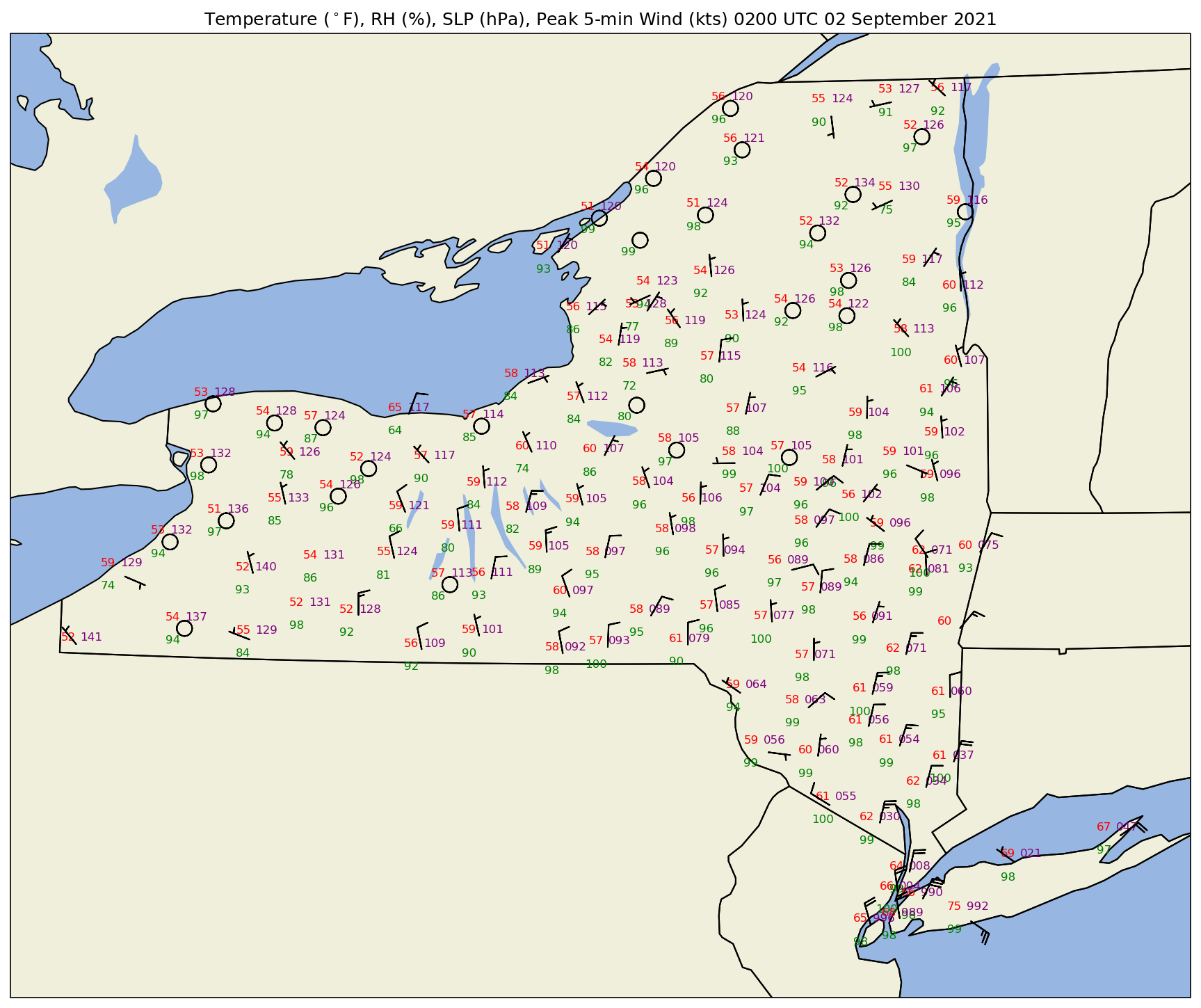
What if we wanted to plot sea-level pressure (SLP) instead of station pressure? In this case, we can apply what’s called a reduction to sea-level pressure formula. This formula requires station elevation (accounting for sensor height) in meters, temperature in Kelvin, and station pressure in hectopascals. We assume each NYSM station has its sensor height .5 meters above ground level.
elev = nysm_sites['elevation']
sensorHeight = .5
# Reduce station pressure to SLP. Source: https://www.sandhurstweather.org.uk/barometric.pdf
slp = pres/np.exp(-1*(elev+sensorHeight)/((tmpc+273.15) * 29.263))
slp
0      1010.929036
1      1007.734534
2      1012.633239
3      1005.404926
4      1008.947468
          ...
121    1013.030846
122    1011.493213
123    1010.712159
124    1011.445598
125    1012.594216
Length: 126, dtype: float64
Make a new map, substituting SLP for station pressure. We will also use the convention of the three least-significant digits to represent SLP in hectopascals.
fig = plt.figure(figsize=(18,12),dpi=150)
ax = fig.add_subplot(1,1,1,projection=proj)
ax.set_extent ([lonW,lonE,latS,latN])
ax.add_feature (cfeature.LAND.with_scale(res))
ax.add_feature (cfeature.OCEAN.with_scale(res))
ax.add_feature(cfeature.COASTLINE.with_scale(res))
ax.add_feature (cfeature.LAKES.with_scale(res))
ax.add_feature (cfeature.STATES.with_scale(res));

# Create a station plot pointing to an Axes to draw on as well as the location of points
stationplot = StationPlot(ax, lons, lats, transform=ccrs.PlateCarree(),
                          fontsize=8)

stationplot.plot_parameter('NW', tmpf, color='red')
stationplot.plot_parameter('SW', rh, color='green')
# A more complex example uses a custom formatter to control how the sea-level pressure
# values are plotted. This uses the standard trailing 3-digits of the pressure value
# in tenths of millibars.
stationplot.plot_parameter('NE', slp, color='purple', formatter=lambda v: format(10 * v, '.0f')[-3:])
stationplot.plot_barb(u, v,zorder=10)
ax.set_title ('Temperature ($^\circ$F), RH (%), SLP (hPa), Peak 5-min Wind (kts) 0200 UTC 02 September 2021');
Summary
Multiple
Seriescan be constructed from multipleDataFramesA single mathematical function can be applied (broadcasted) to all array elements in a
SeriesThe MetPy library provides methods to assign physical units to numerical arrays and perform units-aware calculations
MetPy’s
StationPlotmethod offers a customized use of Matplotlib’s Pyplot library to plot several meteorologically-relevant parameters centered about several geo-referenced points.
What’s Next?
In the next notebook, we will explore several ways in Pandas to reference particular rows, columns, and/or row-column pairs in a Pandas DataFrame.