.ipynb .pdf

repository open issue suggest edit

Contents

Xarray 2: DataArrays

---

Overview

1. Why not use a Pandas DataFrame for gridded data?

2. Anatomy of a DataArray created from a gridded NetCDF data file

Prerequisites

Concepts	Importance	Notes
Python basics	Necessary
Numpy basics	Necessary
Pandas	Necessary
Xarray 1 Intro	Necessary

• Time to learn: 15 minutes

Imports

import xarray as xr
import pandas as pd

Why not use a Pandas DataFrame for gridded data?

Here is a Pandas DataFrame representation of the 500 hPa geopotential height for 0000 UTC 30 October 2012, from the ERA-5 reanalysis:

df = pd.read_csv('/spare11/atm533/data/2012103000_z500_era5.csv',index_col='latitude')

df

	0.0	0.25	0.5	0.75	1.0	1.25	1.5	1.75	2.0	2.25	...	357.5	357.75	358.0	358.25	358.5	358.75	359.0	359.25	359.5	359.75
latitude
90.00	51072.215	51072.215	51072.215	51072.215	51072.215	51072.215	51072.215	51072.215	51072.215	51072.215	...	51072.215	51072.215	51072.215	51072.215	51072.215	51072.215	51072.215	51072.215	51072.215	51072.215
89.75	51049.582	51049.582	51049.746	51049.746	51050.074	51050.074	51050.240	51050.240	51050.566	51050.566	...	51048.270	51048.270	51048.598	51048.598	51048.760	51048.760	51049.090	51049.090	51049.254	51049.254
89.50	51026.950	51027.277	51027.440	51027.770	51028.098	51028.260	51028.590	51028.754	51029.082	51029.246	...	51024.816	51024.980	51025.310	51025.473	51025.800	51025.965	51026.293	51026.293	51026.457	51026.785
89.25	51007.270	51007.598	51008.090	51008.254	51008.582	51009.074	51009.240	51009.566	51009.730	51010.223	...	51004.320	51004.484	51004.810	51005.300	51005.465	51005.793	51005.957	51006.285	51006.777	51006.940
89.00	50990.050	50990.543	50990.707	50991.200	50991.527	50992.020	50992.348	50992.840	50993.004	50993.496	...	50986.770	50987.098	50987.260	50987.754	50988.082	50988.246	50988.740	50989.066	50989.560	50989.723
...	...	...	...	...	...	...	...	...	...	...	...	...	...	...	...	...	...	...	...	...	...
-89.00	48821.510	48821.840	48822.332	48822.496	48822.990	48823.316	48823.480	48823.973	48824.300	48824.465	...	48817.740	48818.230	48818.560	48819.050	48819.215	48819.707	48820.035	48820.527	48820.690	48821.348
-89.25	48783.465	48783.793	48783.957	48784.450	48784.777	48784.940	48785.270	48785.598	48785.758	48786.086	...	48780.840	48781.004	48781.332	48781.496	48781.990	48782.316	48782.480	48782.810	48782.973	48783.300
-89.50	48745.582	48745.582	48745.746	48746.074	48746.074	48746.240	48746.240	48746.562	48746.727	48746.727	...	48743.777	48743.940	48744.270	48744.270	48744.598	48744.760	48744.760	48745.090	48745.090	48745.254
-89.75	48709.500	48709.500	48709.500	48709.500	48709.830	48709.830	48709.830	48709.992	48709.992	48709.992	...	48708.844	48708.844	48708.844	48708.844	48709.008	48709.008	48709.008	48709.336	48709.336	48709.336
-90.00	48673.258	48673.258	48673.258	48673.258	48673.258	48673.258	48673.258	48673.258	48673.258	48673.258	...	48673.258	48673.258	48673.258	48673.258	48673.258	48673.258	48673.258	48673.258	48673.258	48673.258

721 rows × 1440 columns

df.info()

<class 'pandas.core.frame.DataFrame'>
Index: 721 entries, 90.0 to -90.0
Columns: 1440 entries, 0.0 to 359.75
dtypes: float64(1440)
memory usage: 7.9 MB

Output the geopotential height at the grid point closest to Albany (42.75N, -73.75 W; note we have expressed the longitude as if it were degrees East)

df.loc[[42.75],['286.25']]

	286.25
latitude
42.75	53853.285

While Pandas is great for many purposes, extending its inherently 2-d data representation to a multidimensional dataset, such as 4-dimensional (time, vertical level, longitude (x) and latitude (y)) gridded numerical weather prediction (NWP) or c limate model output, is unwise.

Gridded datasets and Xarray

The Xarray package is ideally-suited for gridded data, in particular NetCDF. It builds and extends on the multi-dimensional data structure in NumPy. We will see that some of the same methods we’ve used for Pandas have analogues in Xarray.

Anatomy of a DataArray

Let’s look at the same 500 hPa geopotential height field, but this time we’ll use Xarray to open the NetCDF representation.

da = xr.open_dataarray('/spare11/atm533/data/2012103000_z500_era5.nc')

First, let’s compare the size of gridded field as represented in a plain-text CSV file and in NetCDF.

! ls -lh /spare11/atm533/data/2012103000_z500_era5.csv
! ls -lh /spare11/atm533/data/2012103000_z500_era5.nc

-rw-r--r-- 1 ktyle faculty 9.5M Sep 29  2020 /spare11/atm533/data/2012103000_z500_era5.csv

-rw-r--r-- 1 ktyle faculty 2.0M Sep 29  2020 /spare11/atm533/data/2012103000_z500_era5.nc

The NetCDF-formatted file is smaller. While this particular grid is less than 10 MB either way, the space savings become significant as you scale up!

As did Pandas with its Series and DataFrame core data structures, Xarray also has two “workhorses”: the DataArray and the Dataset. Just as a Pandas DataFrame consists of multiple Series, an Xarray Dataset is made up of DataArray objects. Let’s first look at our DataArray.

# Similar to a Pandas DataFrame, we get a nice (and even more interactive) HTML representation of the object.
da

<xarray.DataArray 'z' (time: 1, latitude: 721, longitude: 1440)>
[1038240 values with dtype=float32]
Coordinates:
  * longitude  (longitude) float32 0.0 0.25 0.5 0.75 ... 359.0 359.2 359.5 359.8
  * latitude   (latitude) float32 90.0 89.75 89.5 89.25 ... -89.5 -89.75 -90.0
  * time       (time) datetime64[ns] 2012-10-30
Attributes:
    units:          m**2 s**-2
    long_name:      Geopotential
    standard_name:  geopotential

xarray.DataArray

'z'

• time: 1
• latitude: 721
• longitude: 1440

• ...

  [1038240 values with dtype=float32]

• Coordinates: (3)
  • longitude
    (longitude)
    float32
    0.0 0.25 0.5 ... 359.2 359.5 359.8

    units :

    degrees_east

    long_name :

    longitude

    array([0.0000e+00, 2.5000e-01, 5.0000e-01, ..., 3.5925e+02, 3.5950e+02,
           3.5975e+02], dtype=float32)

  • latitude
    (latitude)
    float32
    90.0 89.75 89.5 ... -89.75 -90.0

    units :

    degrees_north

    long_name :

    latitude

    array([ 90.  ,  89.75,  89.5 , ..., -89.5 , -89.75, -90.  ], dtype=float32)

  • time
    (time)
    datetime64[ns]
    2012-10-30

    long_name :

    time

    array(['2012-10-30T00:00:00.000000000'], dtype='datetime64[ns]')

• Indexes: (3)
  • longitude
    PandasIndex

    PandasIndex(Index([   0.0,   0.25,    0.5,   0.75,    1.0,   1.25,    1.5,   1.75,    2.0,
             2.25,
           ...
            357.5, 357.75,  358.0, 358.25,  358.5, 358.75,  359.0, 359.25,  359.5,
           359.75],
          dtype='float32', name='longitude', length=1440))

  • latitude
    PandasIndex

    PandasIndex(Index([  90.0,  89.75,   89.5,  89.25,   89.0,  88.75,   88.5,  88.25,   88.0,
            87.75,
           ...
           -87.75,  -88.0, -88.25,  -88.5, -88.75,  -89.0, -89.25,  -89.5, -89.75,
            -90.0],
          dtype='float32', name='latitude', length=721))

  • time
    PandasIndex

    PandasIndex(DatetimeIndex(['2012-10-30'], dtype='datetime64[ns]', name='time', freq=None))

• Attributes: (3)

  units :

  m**2 s**-2

  long_name :

  Geopotential

  standard_name :

  geopotential

---

The DataArray has the following properties:

1. It is a named data variable: ‘z’

2. It has three named dimensions, in order: time, latitude, and longitude.

3. It has three coordinate variables, corresponding to the dimensions.

4. It has attributes which are the data variable’s metadata.

5. Its coordinate variables may have their own metadata as well.

Let’s examine each of these five properties.

1. The data variable, z in this case, is represented by the DataArray object itself. We can query various properties of it, with methods similar to Pandas.

# Akin to column and row indices in Pandas:
da.indexes

Indexes:
    longitude  Index([   0.0,   0.25,    0.5,   0.75,    1.0,   1.25,    1.5,   1.75,    2.0,
         2.25,
       ...
        357.5, 357.75,  358.0, 358.25,  358.5, 358.75,  359.0, 359.25,  359.5,
       359.75],
      dtype='float32', name='longitude', length=1440)
    latitude   Index([  90.0,  89.75,   89.5,  89.25,   89.0,  88.75,   88.5,  88.25,   88.0,
        87.75,
       ...
       -87.75,  -88.0, -88.25,  -88.5, -88.75,  -89.0, -89.25,  -89.5, -89.75,
        -90.0],
      dtype='float32', name='latitude', length=721)
    time       DatetimeIndex(['2012-10-30'], dtype='datetime64[ns]', name='time', freq=None)

da.mean()

<xarray.DataArray 'z' ()>
array(54036.84, dtype=float32)

xarray.DataArray

'z'

• 5.404e+04

  array(54036.84, dtype=float32)

• Coordinates: (0)
• Indexes: (0)
• Attributes: (0)

da.max()

<xarray.DataArray 'z' ()>
array(57970.76953125)

xarray.DataArray

'z'

• 5.797e+04

  array(57970.76953125)

• Coordinates: (0)
• Indexes: (0)
• Attributes: (0)

da.min()

<xarray.DataArray 'z' ()>
array(47223.51953125)

xarray.DataArray

'z'

• 4.722e+04

  array(47223.51953125)

• Coordinates: (0)
• Indexes: (0)
• Attributes: (0)

This invocation will return the lat, lon, and time of the maximum value in the DataArray (source: https://stackoverflow.com/questions/40179593/how-to-get-the-coordinates-of-the-maximum-in-xarray)

da.where(da==da.max(), drop=True).coords

Coordinates:
  * longitude  (longitude) float32 308.5
  * latitude   (latitude) float32 -21.5
  * time       (time) datetime64[ns] 2012-10-30

# We can use loc to select via dimension values, but note that order of indices must follow dimension order. 
da.loc['2012-10-30 00:00',42.75,286.25]

<xarray.DataArray 'z' ()>
array(53853.285, dtype=float32)
Coordinates:
    longitude  float32 286.2
    latitude   float32 42.75
    time       datetime64[ns] 2012-10-30
Attributes:
    units:          m**2 s**-2
    long_name:      Geopotential
    standard_name:  geopotential

xarray.DataArray

'z'

• 5.385e+04

  array(53853.285, dtype=float32)

• Coordinates: (3)
  • longitude
    ()
    float32
    286.2

    units :

    degrees_east

    long_name :

    longitude

    array(286.25, dtype=float32)

  • latitude
    ()
    float32
    42.75

    units :

    degrees_north

    long_name :

    latitude

    array(42.75, dtype=float32)

  • time
    ()
    datetime64[ns]
    2012-10-30

    long_name :

    time

    array('2012-10-30T00:00:00.000000000', dtype='datetime64[ns]')

• Indexes: (0)
• Attributes: (3)

  units :

  m**2 s**-2

  long_name :

  Geopotential

  standard_name :

  geopotential

We can alternatively use Xarray’s sel indexing technique, where we specify the names of the dimension and the values we are selecting … can be in any order.

da.sel(latitude=42.75, longitude = 286.25)

<xarray.DataArray 'z' (time: 1)>
array([53853.285], dtype=float32)
Coordinates:
    longitude  float32 286.2
    latitude   float32 42.75
  * time       (time) datetime64[ns] 2012-10-30
Attributes:
    units:          m**2 s**-2
    long_name:      Geopotential
    standard_name:  geopotential

xarray.DataArray

'z'

• time: 1

• 5.385e+04

  array([53853.285], dtype=float32)

• Coordinates: (3)
  • longitude
    ()
    float32
    286.2

    units :

    degrees_east

    long_name :

    longitude

    array(286.25, dtype=float32)

  • latitude
    ()
    float32
    42.75

    units :

    degrees_north

    long_name :

    latitude

    array(42.75, dtype=float32)

  • time
    (time)
    datetime64[ns]
    2012-10-30

    long_name :

    time

    array(['2012-10-30T00:00:00.000000000'], dtype='datetime64[ns]')

• Indexes: (1)
  • time
    PandasIndex

    PandasIndex(DatetimeIndex(['2012-10-30'], dtype='datetime64[ns]', name='time', freq=None))

• Attributes: (3)

  units :

  m**2 s**-2

  long_name :

  Geopotential

  standard_name :

  geopotential

2. Dimension names

In Xarray, dimensions can be thought of as extensions of Pandas’ 2-d row/column indices (aka axes). We can assign names, or labels, to Pandas indexes; in Xarray, these labeled axes are a necessary (and excellent) feature.

da.dims

('time', 'latitude', 'longitude')

3. Coordinates

Coordinate variables in Xarray are 1-dimensional arrays that correspond to the Data variable’s dimensions. In this case, z has dimension coordinates of longitude, latitude, and time; each of these three dimension coordinates consist of an array of values, plus metadata.

da.coords

Coordinates:
  * longitude  (longitude) float32 0.0 0.25 0.5 0.75 ... 359.0 359.2 359.5 359.8
  * latitude   (latitude) float32 90.0 89.75 89.5 89.25 ... -89.5 -89.75 -90.0
  * time       (time) datetime64[ns] 2012-10-30

We can assign an object to each coordinate dimension.

lons = da.longitude

lats = da.latitude

times = da.time

lons

<xarray.DataArray 'longitude' (longitude: 1440)>
array([0.0000e+00, 2.5000e-01, 5.0000e-01, ..., 3.5925e+02, 3.5950e+02,
       3.5975e+02], dtype=float32)
Coordinates:
  * longitude  (longitude) float32 0.0 0.25 0.5 0.75 ... 359.0 359.2 359.5 359.8
Attributes:
    units:      degrees_east
    long_name:  longitude

xarray.DataArray

'longitude'

• longitude: 1440

• 0.0 0.25 0.5 0.75 1.0 1.25 1.5 ... 358.5 358.8 359.0 359.2 359.5 359.8

  array([0.0000e+00, 2.5000e-01, 5.0000e-01, ..., 3.5925e+02, 3.5950e+02,
         3.5975e+02], dtype=float32)

• Coordinates: (1)
  • longitude
    (longitude)
    float32
    0.0 0.25 0.5 ... 359.2 359.5 359.8

    units :

    degrees_east

    long_name :

    longitude

    array([0.0000e+00, 2.5000e-01, 5.0000e-01, ..., 3.5925e+02, 3.5950e+02,
           3.5975e+02], dtype=float32)

• Indexes: (1)
  • longitude
    PandasIndex

    PandasIndex(Index([   0.0,   0.25,    0.5,   0.75,    1.0,   1.25,    1.5,   1.75,    2.0,
             2.25,
           ...
            357.5, 357.75,  358.0, 358.25,  358.5, 358.75,  359.0, 359.25,  359.5,
           359.75],
          dtype='float32', name='longitude', length=1440))

• Attributes: (2)

  units :

  degrees_east

  long_name :

  longitude

4. The data variables will typically have attributes (metadata) attached to them.

da.attrs

{'units': 'm**2 s**-2',
 'long_name': 'Geopotential',
 'standard_name': 'geopotential'}

da.units

'm**2 s**-2'

5. The coordinate variables will likely have metadata as well.

times.attrs

{'long_name': 'time'}

lats.attrs

{'units': 'degrees_north', 'long_name': 'latitude'}

Just as with Pandas, Xarray has a built-in hook to Matplotlib so we can take a quick look at our data.

da.plot()

<matplotlib.collections.QuadMesh at 0x14dc3c551810>

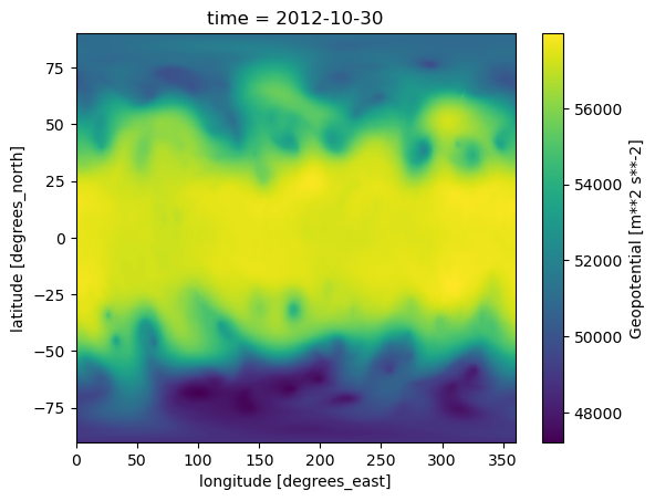
This NetCDF file that we read in had just a single data variable … one time, at one vertical level. Typically, gridded model or reanalysis data in NetCDF format will consist of multiple variables … i.e., multiple Xarray DataArrays … known as a Dataset. In the rest of our Xarray notebooks, we will read in, analyze, and visualize examples of Datasets.

---

Summary

• Xarray builds upon the data models provided by NumPy and Pandas.

• Xarray provides read and write methods for a variety of gridded datasets, such as NetCDF, GRIB, and Zarr.

• Xarray Datasets consist of one or more `DataArrays’.

• A DataArray typically contains one data variable, with labeled dimensions and coordinates.

What’s Next?

In the next notebook, we’ll work with an Xarray Dataset and make some plots from it.

Resources and References

1. Xarray Documentation

2. SciPy 2020 Xarray Tutorial

previous

Xarray 1: Introduction to Xarray

next

Xarray 3: Datasets and Plotting