Rasters 3: Cloud-optimized GeoTIFFs with multiple bands¶

Overview¶

Read in a high-resolution, cloud-optimized GeoTIFF that consists of multiple bands
Combine the bands into a single, true-color image and plot that image
Overlay the GeoTIFF on GeoAxes

Prerequisites¶

Concepts	Importance	Notes
Rasters 1-2	Necessary

Time to learn: 30 minutes

Imports¶

import matplotlib.pyplot as plt
import cartopy.crs as ccrs
import cartopy.feature as cfeature
import numpy as np
import rioxarray as rxr
import rasterio

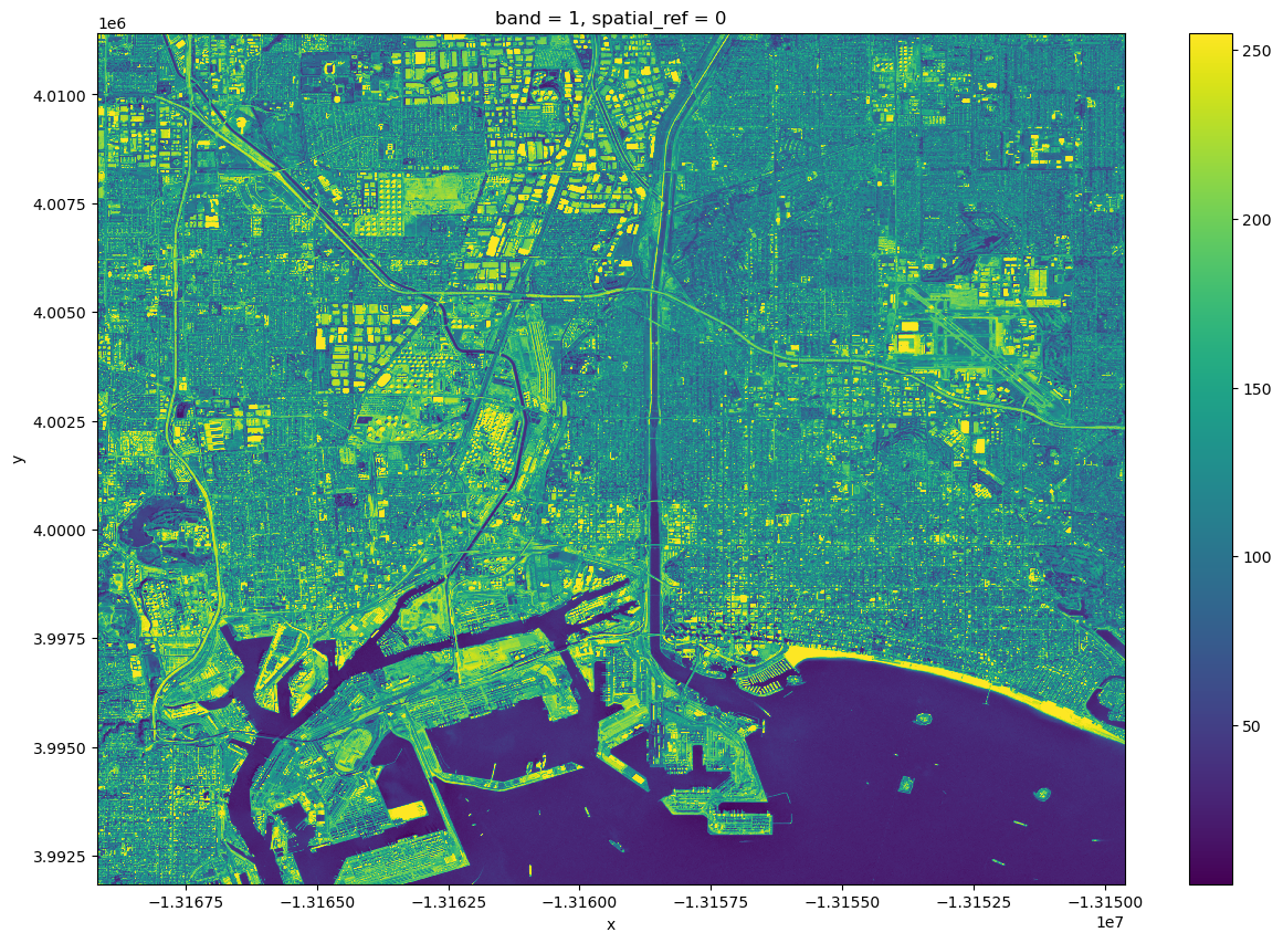
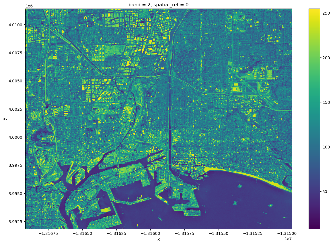
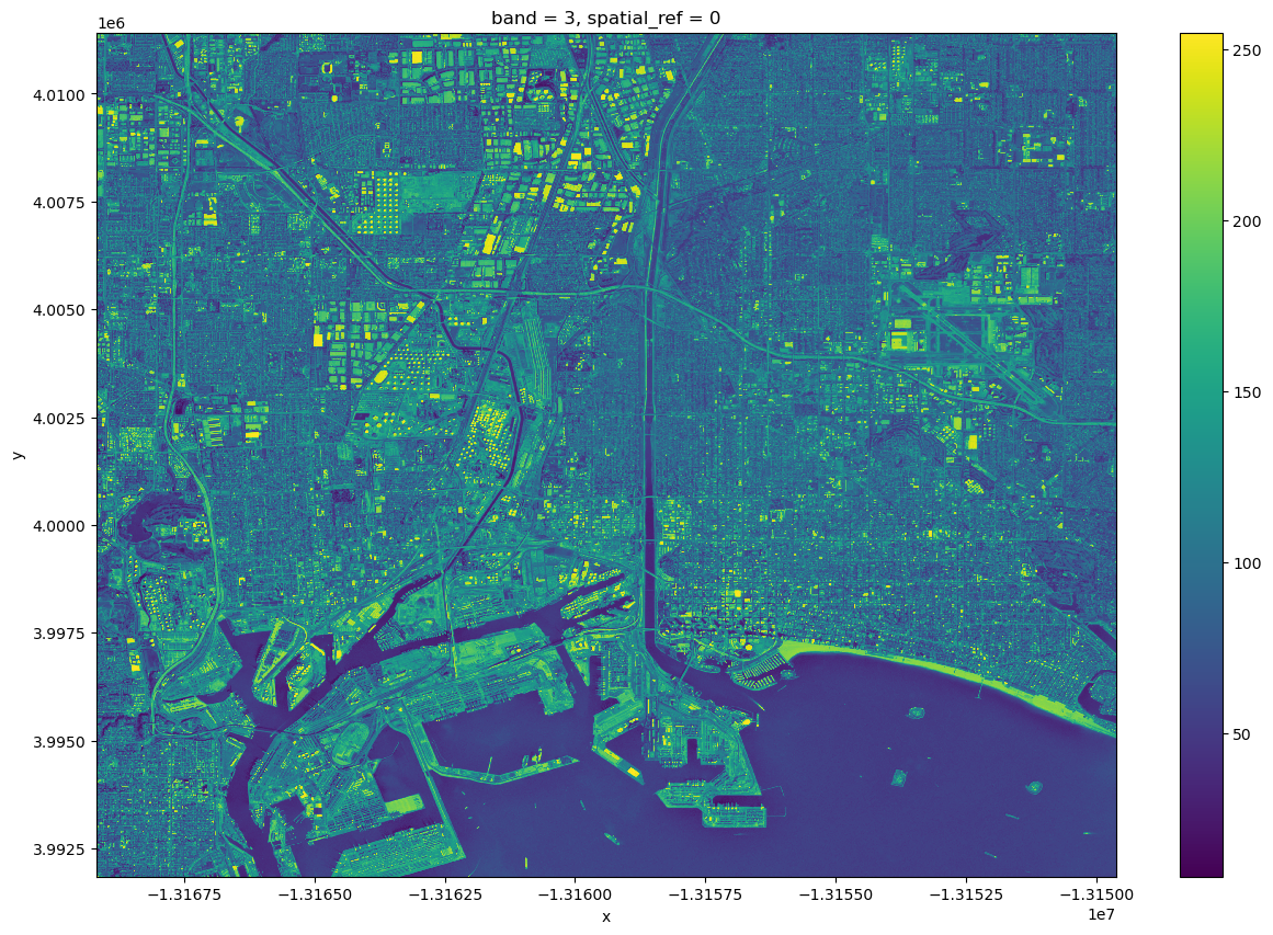
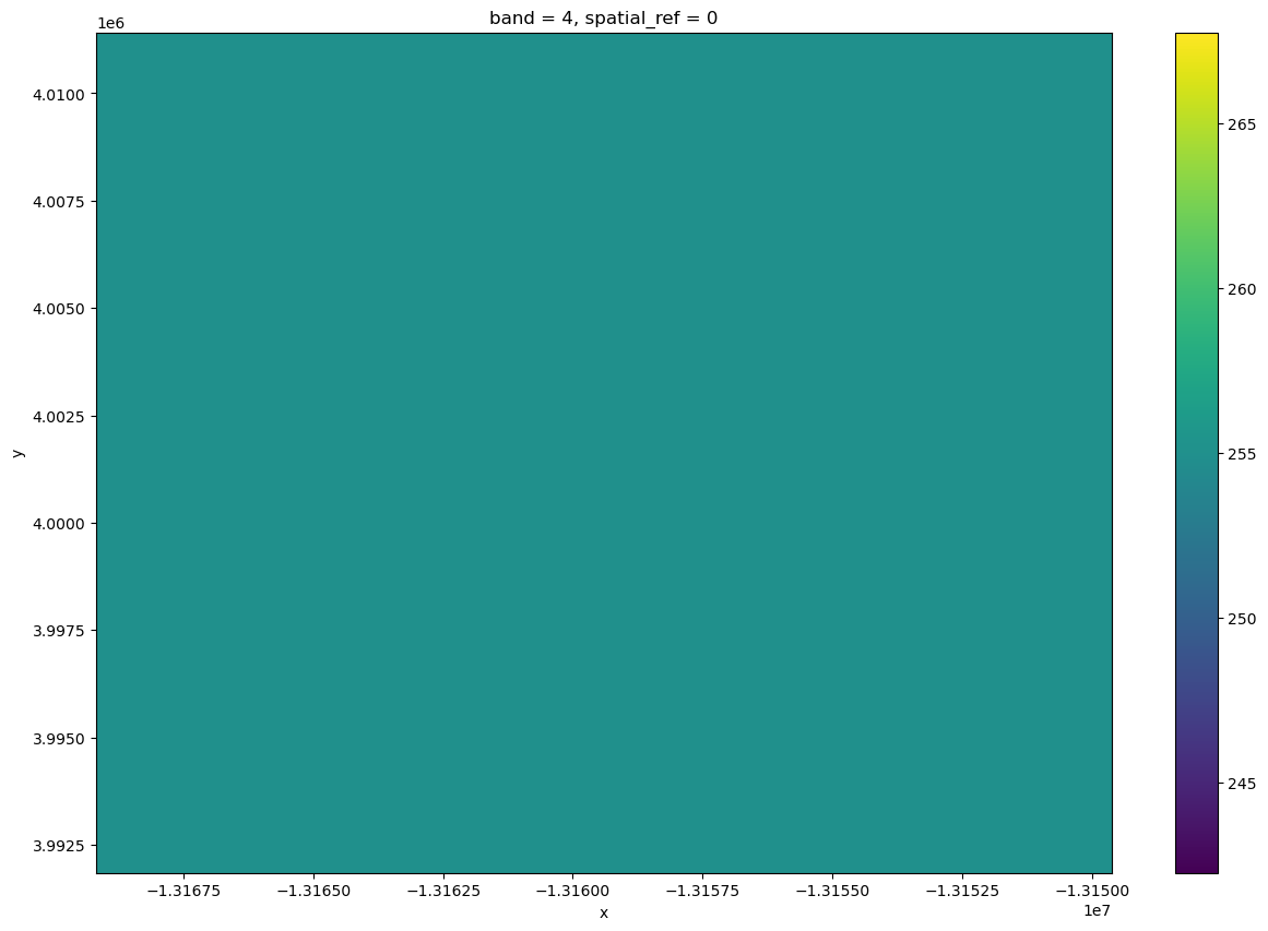
Plot each of the bands directly from Xarray.¶

figSize = (15,10)

for n in range(1,5):
    cog.sel(band=n).plot.imshow(figsize=figSize)

../../_images/e5bc19be432adc93551eefd6dc645b38385f6662092eeee87a2d83cf362d3498.png

../../_images/317fd9de1e30510706baf622319030eea48dc1cf3c132a79b4105e62a1d1fcb8.png

../../_images/3c33074dba6df0e5d418a255a748b59739933b6dc1877fd8d391540f5099a62d.png

../../_images/f111c99c7c1cd7c9d34604a3f45472c2a24edd88e65b106c96ad3ff05763aacd.png

Note: Notice that a default colormap was used, and while we can certainly discern salient features of the underlying surface, the applied colors are deceptive. The four bands are actually red, green, blue, and alpha (transparency) pixel values (commonly termed RGBA). For this imagery, alpha = 0 signifies missing data (and there are no missing data points).

Close this Xarray DataArray as we’re done with it for now.

cog.close()

Combine the bands into a single, true-color image¶

We will now use the more general rasterio library to deal with combining these bands into a single image.

Stack together the first 3 RGB bands to arrive at a true-color composite image (see refs. 3 and 4 at end of notebook).

Note: By default, rasterio assumes that a GeoTIFF with 3 bands has a band order of red, green and blue (RGB). It interprets a 4-band image as RGB/A, where *A* denotes *alpha*, or transparency. Each of these four bands, or channels, have pixel values ranging from 0 to 255. For the three colors, the range goes from no color to saturated (full) color. For alpha, the range goes from completely transparent to completely opaque.

Rasterio’s colorinterp method will display how it is characterizing each of these channels. The following cell demonstrates the procedure:

with rasterio.open(rasFile) as src:
    # convert / read the data into a numpy array:
    cog = src.read(masked= True)
    red = src.read(1)
    green = src.read(2)
    blue = src.read(3)
    print(src.colorinterp[0])
    print(src.colorinterp[1])
    print(src.colorinterp[2])
    print(src.colorinterp[3])

cog.shape

(4, 4096, 4096)

Notice that cog has 3 dimensions.

Now, create a function to normalize each of the three RGB bands so the ranges are from 0 to 1. We will ignore the alpha channel; for this GeoTIFF, alpha is set to 0 only for missing points, of which there are none.

def normalize(array):
    array_min, array_max = array.min(), array.max()
    return (array - array_min) / (array_max - array_min)

Normalize the RGB bands

red_norm = normalize(red)
green_norm = normalize(green)
blue_norm = normalize(blue)

Note: Each of these are NumPy arrays; we can use NumPy's dstack function to create a single NumPy array that now has all three channels. This is known as a true color image.

rgb = np.dstack((red_norm, green_norm, blue_norm))

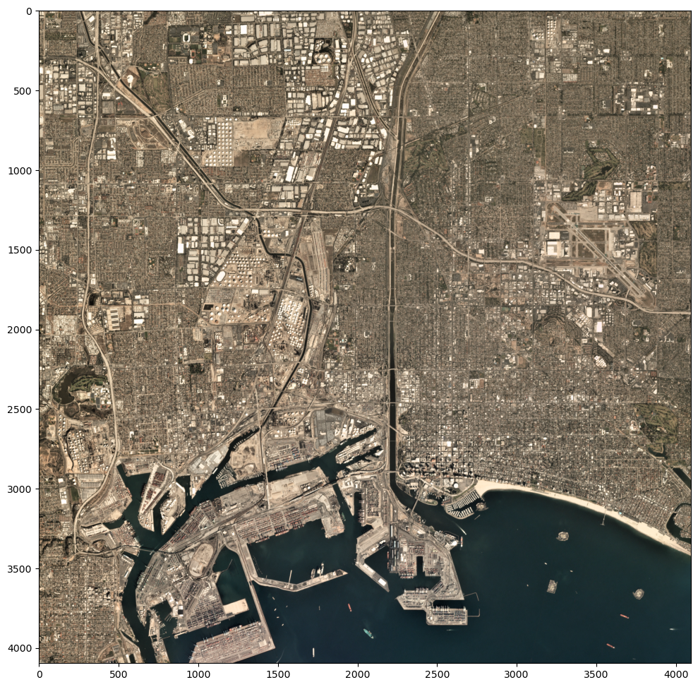
Visualize the true-color image.¶

To start, we will not create geo-referenced Matplotlib axes with Cartopy … we’ll do that shortly.

fig = plt.figure(figsize=(18,12))
plt.imshow(rgb);

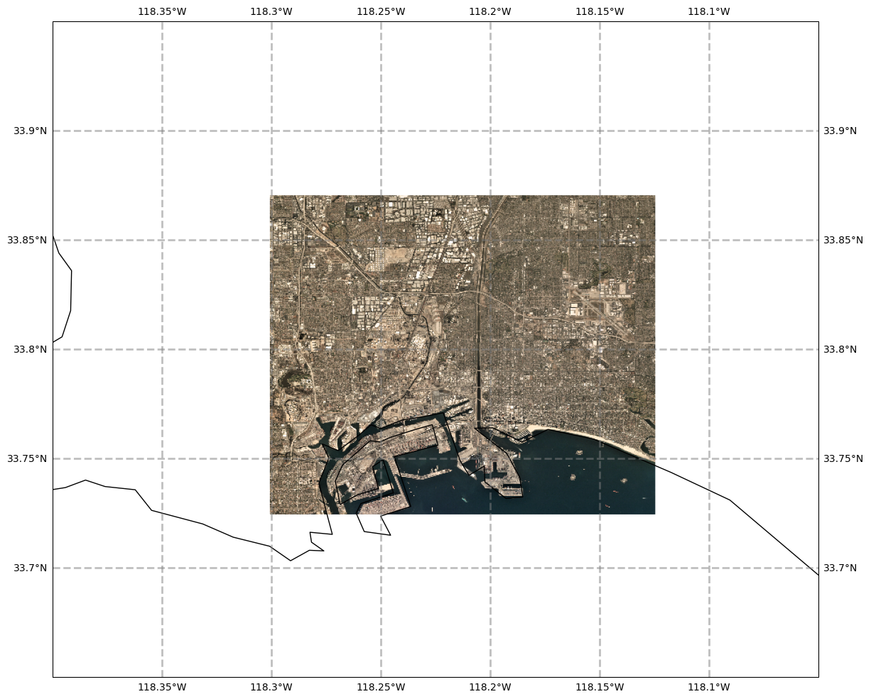
../../_images/54b66436f55c9ba85cd1638f16672ce328bddd41bb0bbdaac67ba128c3b76921.png

Overlay the GeoTIFF on GeoAxes¶

Now, let’s plot this image on a set of GeoAxes. We’ll include the NaturalEarth high-res coastline shapefile which will help show how much of the plotted area is encompassed by the true-color image.

res = '10m'
fig = plt.figure(figsize=(18,12))
ax = plt.subplot(1,1,1,projection=ccrs.PlateCarree())
ax.set_extent((-118.4,-118.05,33.65,33.95),crs=ccrs.PlateCarree())
ax.gridlines(draw_labels=True,
                  linewidth=2, color='gray', alpha=0.5, linestyle='--')
ax.add_feature(cfeature.COASTLINE.with_scale(res))
im = ax.imshow(rgb,extent=[left, right, bottom, top],transform=projCOG)

../../_images/253dfae8311f77b931a485d051cd5a89600bd06b0c3836faad0033042807af04.png

Note: If you've ever used the Satellite option in Google Maps, you've no doubt seen imagery like this! In this case, we have just one small (~ 20km x 20km), but very hi-res raster image. This single image and its neighbors get loaded in as image tiles by interactive mapping applications that one can zoom into or out of. By virtue of these images being in cloud-optimized GeoTIFF format, the downloading of the tiles and creation / rendering of the mosaics can occur very quickly!

To think about: We've already overlaid raster data on GeoTIFFs. With such high-resolution imagery such as the Los Angeles tile above, consider the utility of plotting *point-based* data over similar imagery. Coming soon, we'll work with geo-referenced Pandas Dataframes, and plot the location of lightning strikes over a GeoTIFF.

Summary¶

Geo-referenced GeoTIFFs typically consist of three (RGB) or four (RGBA) bands.
Via the rioxarray library, these bands make up the data variables when opened as a Xarray Dataset.
GeoTIFFs that are optimized for cloud storage are called Cloud-optimized GeoTIFFs (COGs).
Just like any geo-referenced array, COGs can be visualized with Matplotlib and Cartopy.

What’s Next?¶

Raster and vector data are the two core datatypes used in GIS. We’ll next explore vector data, which include shapefiles.

ATM433/533 Fall 2023

Rasters 3: Cloud-optimized GeoTIFFs with multiple bands

Contents