Xarray 7: Calculating ENSO with Xarray
Contents
Xarray 7: Calculating ENSO with Xarray
Objectives
Load SST data from CESM2
Mask data using
.where()methodCompute climatologies and anomalies using
.groupby()Use
.rolling()to compute moving averageCompute, normalize, and plot the Niño 3.4 Index
Prerequisites
Concepts |
Importance |
Notes |
|---|---|---|
Introduction to Xarray |
Necessary |
|
Computation and Masking |
Necessary |
Time to learn: 20 minutes
Imports
import cartopy.crs as ccrs
import matplotlib.pyplot as plt
import xarray as xr
from pythia_datasets import DATASETS
Niño 3.4 Index
In this notebook, we are going to combine all concepts/topics we’ve covered so far to compute Niño 3.4 Index for the CESM2 submission for the CMIP6 project.
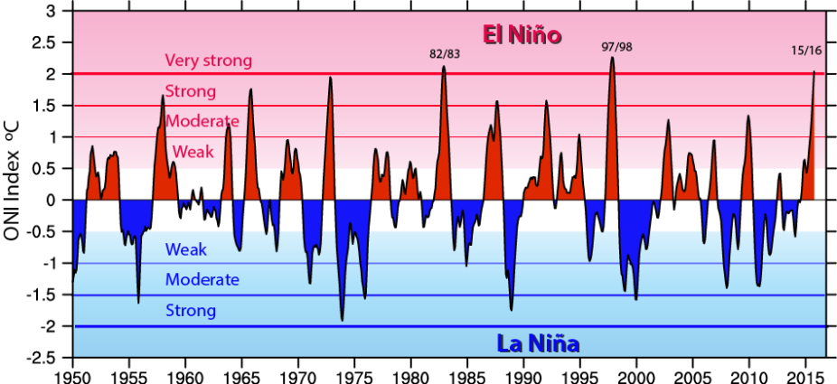
Niño 3.4 (5N-5S, 170W-120W): The Niño 3.4 anomalies may be thought of as representing the average equatorial SSTs across the Pacific from about the dateline to the South American coast. The Niño 3.4 index typically uses a 5-month running mean, and El Niño or La Niña events are defined when the Niño 3.4 SSTs exceed +/- 0.4C for a period of six months or more.
Nino X Index computation: (a) Compute area averaged total SST from Niño X region; (b) Compute monthly climatology (e.g., 1950-1979) for area averaged total SST from Niño X region, and subtract climatology from area averaged total SST time series to obtain anomalies; © Smooth the anomalies with a 5-month running mean; (d) Normalize the smoothed values by its standard deviation over the climatological period.
At the end of this notebook, you should be able to produce a plot that looks similar to this Oceanic Niño Index plot:
Open the sea surface temperature and areacello datasets and use Xarray’s merge method to combine them into a single one.
filepath = DATASETS.fetch('CESM2_sst_data.nc')
data = xr.open_dataset(filepath)
filepath2 = DATASETS.fetch('CESM2_grid_variables.nc')
areacello = xr.open_dataset(filepath2).areacello
ds = xr.merge([data, areacello])
ds
<xarray.Dataset>
Dimensions:    (time: 180, d2: 2, lat: 180, lon: 360)
Coordinates:
  * time       (time) object 2000-01-15 12:00:00 ... 2014-12-15 12:00:00
  * lat        (lat) float64 -89.5 -88.5 -87.5 -86.5 ... 86.5 87.5 88.5 89.5
  * lon        (lon) float64 0.5 1.5 2.5 3.5 4.5 ... 356.5 357.5 358.5 359.5
Dimensions without coordinates: d2
Data variables:
    time_bnds  (time, d2) object ...
    lat_bnds   (lat, d2) float64 ...
    lon_bnds   (lon, d2) float64 ...
    tos        (time, lat, lon) float32 ...
    areacello  (lat, lon) float64 ...
Attributes: (12/45)
    Conventions:            CF-1.7 CMIP-6.2
    activity_id:            CMIP
    branch_method:          standard
    branch_time_in_child:   674885.0
    branch_time_in_parent:  219000.0
    case_id:                972
    ...                     ...
    sub_experiment_id:      none
    table_id:               Omon
    tracking_id:            hdl:21.14100/2975ffd3-1d7b-47e3-961a-33f212ea4eb2
    variable_id:            tos
    variant_info:           CMIP6 20th century experiments (1850-2014) with C...
variant_label: r11i1p1f1- time: 180
- d2: 2
- lat: 180
- lon: 360
- time(time)object2000-01-15 12:00:00 ... 2014-12-...
- axis :
- T
- bounds :
- time_bnds
- standard_name :
- time
- title :
- time
- type :
- double
array([cftime.DatetimeNoLeap(2000, 1, 15, 12, 0, 0, 0, has_year_zero=True), cftime.DatetimeNoLeap(2000, 2, 14, 0, 0, 0, 0, has_year_zero=True), cftime.DatetimeNoLeap(2000, 3, 15, 12, 0, 0, 0, has_year_zero=True), cftime.DatetimeNoLeap(2000, 4, 15, 0, 0, 0, 0, has_year_zero=True), cftime.DatetimeNoLeap(2000, 5, 15, 12, 0, 0, 0, has_year_zero=True), cftime.DatetimeNoLeap(2000, 6, 15, 0, 0, 0, 0, has_year_zero=True), cftime.DatetimeNoLeap(2000, 7, 15, 12, 0, 0, 0, has_year_zero=True), cftime.DatetimeNoLeap(2000, 8, 15, 12, 0, 0, 0, has_year_zero=True), cftime.DatetimeNoLeap(2000, 9, 15, 0, 0, 0, 0, has_year_zero=True), cftime.DatetimeNoLeap(2000, 10, 15, 12, 0, 0, 0, has_year_zero=True), cftime.DatetimeNoLeap(2000, 11, 15, 0, 0, 0, 0, has_year_zero=True), cftime.DatetimeNoLeap(2000, 12, 15, 12, 0, 0, 0, has_year_zero=True), cftime.DatetimeNoLeap(2001, 1, 15, 12, 0, 0, 0, has_year_zero=True), cftime.DatetimeNoLeap(2001, 2, 14, 0, 0, 0, 0, has_year_zero=True), cftime.DatetimeNoLeap(2001, 3, 15, 12, 0, 0, 0, has_year_zero=True), cftime.DatetimeNoLeap(2001, 4, 15, 0, 0, 0, 0, has_year_zero=True), cftime.DatetimeNoLeap(2001, 5, 15, 12, 0, 0, 0, has_year_zero=True), cftime.DatetimeNoLeap(2001, 6, 15, 0, 0, 0, 0, has_year_zero=True), cftime.DatetimeNoLeap(2001, 7, 15, 12, 0, 0, 0, has_year_zero=True), cftime.DatetimeNoLeap(2001, 8, 15, 12, 0, 0, 0, has_year_zero=True), cftime.DatetimeNoLeap(2001, 9, 15, 0, 0, 0, 0, has_year_zero=True), cftime.DatetimeNoLeap(2001, 10, 15, 12, 0, 0, 0, has_year_zero=True), cftime.DatetimeNoLeap(2001, 11, 15, 0, 0, 0, 0, has_year_zero=True), cftime.DatetimeNoLeap(2001, 12, 15, 12, 0, 0, 0, has_year_zero=True), cftime.DatetimeNoLeap(2002, 1, 15, 12, 0, 0, 0, has_year_zero=True), cftime.DatetimeNoLeap(2002, 2, 14, 0, 0, 0, 0, has_year_zero=True), cftime.DatetimeNoLeap(2002, 3, 15, 12, 0, 0, 0, has_year_zero=True), cftime.DatetimeNoLeap(2002, 4, 15, 0, 0, 0, 0, has_year_zero=True), cftime.DatetimeNoLeap(2002, 5, 15, 12, 0, 0, 0, has_year_zero=True), cftime.DatetimeNoLeap(2002, 6, 15, 0, 0, 0, 0, has_year_zero=True), cftime.DatetimeNoLeap(2002, 7, 15, 12, 0, 0, 0, has_year_zero=True), cftime.DatetimeNoLeap(2002, 8, 15, 12, 0, 0, 0, has_year_zero=True), cftime.DatetimeNoLeap(2002, 9, 15, 0, 0, 0, 0, has_year_zero=True), cftime.DatetimeNoLeap(2002, 10, 15, 12, 0, 0, 0, has_year_zero=True), cftime.DatetimeNoLeap(2002, 11, 15, 0, 0, 0, 0, has_year_zero=True), cftime.DatetimeNoLeap(2002, 12, 15, 12, 0, 0, 0, has_year_zero=True), cftime.DatetimeNoLeap(2003, 1, 15, 12, 0, 0, 0, has_year_zero=True), cftime.DatetimeNoLeap(2003, 2, 14, 0, 0, 0, 0, has_year_zero=True), cftime.DatetimeNoLeap(2003, 3, 15, 12, 0, 0, 0, has_year_zero=True), cftime.DatetimeNoLeap(2003, 4, 15, 0, 0, 0, 0, has_year_zero=True), cftime.DatetimeNoLeap(2003, 5, 15, 12, 0, 0, 0, has_year_zero=True), cftime.DatetimeNoLeap(2003, 6, 15, 0, 0, 0, 0, has_year_zero=True), cftime.DatetimeNoLeap(2003, 7, 15, 12, 0, 0, 0, has_year_zero=True), cftime.DatetimeNoLeap(2003, 8, 15, 12, 0, 0, 0, has_year_zero=True), cftime.DatetimeNoLeap(2003, 9, 15, 0, 0, 0, 0, has_year_zero=True), cftime.DatetimeNoLeap(2003, 10, 15, 12, 0, 0, 0, has_year_zero=True), cftime.DatetimeNoLeap(2003, 11, 15, 0, 0, 0, 0, has_year_zero=True), cftime.DatetimeNoLeap(2003, 12, 15, 12, 0, 0, 0, has_year_zero=True), cftime.DatetimeNoLeap(2004, 1, 15, 12, 0, 0, 0, has_year_zero=True), cftime.DatetimeNoLeap(2004, 2, 14, 0, 0, 0, 0, has_year_zero=True), cftime.DatetimeNoLeap(2004, 3, 15, 12, 0, 0, 0, has_year_zero=True), cftime.DatetimeNoLeap(2004, 4, 15, 0, 0, 0, 0, has_year_zero=True), cftime.DatetimeNoLeap(2004, 5, 15, 12, 0, 0, 0, has_year_zero=True), cftime.DatetimeNoLeap(2004, 6, 15, 0, 0, 0, 0, has_year_zero=True), cftime.DatetimeNoLeap(2004, 7, 15, 12, 0, 0, 0, has_year_zero=True), cftime.DatetimeNoLeap(2004, 8, 15, 12, 0, 0, 0, has_year_zero=True), cftime.DatetimeNoLeap(2004, 9, 15, 0, 0, 0, 0, has_year_zero=True), cftime.DatetimeNoLeap(2004, 10, 15, 12, 0, 0, 0, has_year_zero=True), cftime.DatetimeNoLeap(2004, 11, 15, 0, 0, 0, 0, has_year_zero=True), cftime.DatetimeNoLeap(2004, 12, 15, 12, 0, 0, 0, has_year_zero=True), cftime.DatetimeNoLeap(2005, 1, 15, 12, 0, 0, 0, has_year_zero=True), cftime.DatetimeNoLeap(2005, 2, 14, 0, 0, 0, 0, has_year_zero=True), cftime.DatetimeNoLeap(2005, 3, 15, 12, 0, 0, 0, has_year_zero=True), cftime.DatetimeNoLeap(2005, 4, 15, 0, 0, 0, 0, has_year_zero=True), cftime.DatetimeNoLeap(2005, 5, 15, 12, 0, 0, 0, has_year_zero=True), cftime.DatetimeNoLeap(2005, 6, 15, 0, 0, 0, 0, has_year_zero=True), cftime.DatetimeNoLeap(2005, 7, 15, 12, 0, 0, 0, has_year_zero=True), cftime.DatetimeNoLeap(2005, 8, 15, 12, 0, 0, 0, has_year_zero=True), cftime.DatetimeNoLeap(2005, 9, 15, 0, 0, 0, 0, has_year_zero=True), cftime.DatetimeNoLeap(2005, 10, 15, 12, 0, 0, 0, has_year_zero=True), cftime.DatetimeNoLeap(2005, 11, 15, 0, 0, 0, 0, has_year_zero=True), cftime.DatetimeNoLeap(2005, 12, 15, 12, 0, 0, 0, has_year_zero=True), cftime.DatetimeNoLeap(2006, 1, 15, 12, 0, 0, 0, has_year_zero=True), cftime.DatetimeNoLeap(2006, 2, 14, 0, 0, 0, 0, has_year_zero=True), cftime.DatetimeNoLeap(2006, 3, 15, 12, 0, 0, 0, has_year_zero=True), cftime.DatetimeNoLeap(2006, 4, 15, 0, 0, 0, 0, has_year_zero=True), cftime.DatetimeNoLeap(2006, 5, 15, 12, 0, 0, 0, has_year_zero=True), cftime.DatetimeNoLeap(2006, 6, 15, 0, 0, 0, 0, has_year_zero=True), cftime.DatetimeNoLeap(2006, 7, 15, 12, 0, 0, 0, has_year_zero=True), cftime.DatetimeNoLeap(2006, 8, 15, 12, 0, 0, 0, has_year_zero=True), cftime.DatetimeNoLeap(2006, 9, 15, 0, 0, 0, 0, has_year_zero=True), cftime.DatetimeNoLeap(2006, 10, 15, 12, 0, 0, 0, has_year_zero=True), cftime.DatetimeNoLeap(2006, 11, 15, 0, 0, 0, 0, has_year_zero=True), cftime.DatetimeNoLeap(2006, 12, 15, 12, 0, 0, 0, has_year_zero=True), cftime.DatetimeNoLeap(2007, 1, 15, 12, 0, 0, 0, has_year_zero=True), cftime.DatetimeNoLeap(2007, 2, 14, 0, 0, 0, 0, has_year_zero=True), cftime.DatetimeNoLeap(2007, 3, 15, 12, 0, 0, 0, has_year_zero=True), cftime.DatetimeNoLeap(2007, 4, 15, 0, 0, 0, 0, has_year_zero=True), cftime.DatetimeNoLeap(2007, 5, 15, 12, 0, 0, 0, has_year_zero=True), cftime.DatetimeNoLeap(2007, 6, 15, 0, 0, 0, 0, has_year_zero=True), cftime.DatetimeNoLeap(2007, 7, 15, 12, 0, 0, 0, has_year_zero=True), cftime.DatetimeNoLeap(2007, 8, 15, 12, 0, 0, 0, has_year_zero=True), cftime.DatetimeNoLeap(2007, 9, 15, 0, 0, 0, 0, has_year_zero=True), cftime.DatetimeNoLeap(2007, 10, 15, 12, 0, 0, 0, has_year_zero=True), cftime.DatetimeNoLeap(2007, 11, 15, 0, 0, 0, 0, has_year_zero=True), cftime.DatetimeNoLeap(2007, 12, 15, 12, 0, 0, 0, has_year_zero=True), cftime.DatetimeNoLeap(2008, 1, 15, 12, 0, 0, 0, has_year_zero=True), cftime.DatetimeNoLeap(2008, 2, 14, 0, 0, 0, 0, has_year_zero=True), cftime.DatetimeNoLeap(2008, 3, 15, 12, 0, 0, 0, has_year_zero=True), cftime.DatetimeNoLeap(2008, 4, 15, 0, 0, 0, 0, has_year_zero=True), cftime.DatetimeNoLeap(2008, 5, 15, 12, 0, 0, 0, has_year_zero=True), cftime.DatetimeNoLeap(2008, 6, 15, 0, 0, 0, 0, has_year_zero=True), cftime.DatetimeNoLeap(2008, 7, 15, 12, 0, 0, 0, has_year_zero=True), cftime.DatetimeNoLeap(2008, 8, 15, 12, 0, 0, 0, has_year_zero=True), cftime.DatetimeNoLeap(2008, 9, 15, 0, 0, 0, 0, has_year_zero=True), cftime.DatetimeNoLeap(2008, 10, 15, 12, 0, 0, 0, has_year_zero=True), cftime.DatetimeNoLeap(2008, 11, 15, 0, 0, 0, 0, has_year_zero=True), cftime.DatetimeNoLeap(2008, 12, 15, 12, 0, 0, 0, has_year_zero=True), cftime.DatetimeNoLeap(2009, 1, 15, 12, 0, 0, 0, has_year_zero=True), cftime.DatetimeNoLeap(2009, 2, 14, 0, 0, 0, 0, has_year_zero=True), cftime.DatetimeNoLeap(2009, 3, 15, 12, 0, 0, 0, has_year_zero=True), cftime.DatetimeNoLeap(2009, 4, 15, 0, 0, 0, 0, has_year_zero=True), cftime.DatetimeNoLeap(2009, 5, 15, 12, 0, 0, 0, has_year_zero=True), cftime.DatetimeNoLeap(2009, 6, 15, 0, 0, 0, 0, has_year_zero=True), cftime.DatetimeNoLeap(2009, 7, 15, 12, 0, 0, 0, has_year_zero=True), cftime.DatetimeNoLeap(2009, 8, 15, 12, 0, 0, 0, has_year_zero=True), cftime.DatetimeNoLeap(2009, 9, 15, 0, 0, 0, 0, has_year_zero=True), cftime.DatetimeNoLeap(2009, 10, 15, 12, 0, 0, 0, has_year_zero=True), cftime.DatetimeNoLeap(2009, 11, 15, 0, 0, 0, 0, has_year_zero=True), cftime.DatetimeNoLeap(2009, 12, 15, 12, 0, 0, 0, has_year_zero=True), cftime.DatetimeNoLeap(2010, 1, 15, 12, 0, 0, 0, has_year_zero=True), cftime.DatetimeNoLeap(2010, 2, 14, 0, 0, 0, 0, has_year_zero=True), cftime.DatetimeNoLeap(2010, 3, 15, 12, 0, 0, 0, has_year_zero=True), cftime.DatetimeNoLeap(2010, 4, 15, 0, 0, 0, 0, has_year_zero=True), cftime.DatetimeNoLeap(2010, 5, 15, 12, 0, 0, 0, has_year_zero=True), cftime.DatetimeNoLeap(2010, 6, 15, 0, 0, 0, 0, has_year_zero=True), cftime.DatetimeNoLeap(2010, 7, 15, 12, 0, 0, 0, has_year_zero=True), cftime.DatetimeNoLeap(2010, 8, 15, 12, 0, 0, 0, has_year_zero=True), cftime.DatetimeNoLeap(2010, 9, 15, 0, 0, 0, 0, has_year_zero=True), cftime.DatetimeNoLeap(2010, 10, 15, 12, 0, 0, 0, has_year_zero=True), cftime.DatetimeNoLeap(2010, 11, 15, 0, 0, 0, 0, has_year_zero=True), cftime.DatetimeNoLeap(2010, 12, 15, 12, 0, 0, 0, has_year_zero=True), cftime.DatetimeNoLeap(2011, 1, 15, 12, 0, 0, 0, has_year_zero=True), cftime.DatetimeNoLeap(2011, 2, 14, 0, 0, 0, 0, has_year_zero=True), cftime.DatetimeNoLeap(2011, 3, 15, 12, 0, 0, 0, has_year_zero=True), cftime.DatetimeNoLeap(2011, 4, 15, 0, 0, 0, 0, has_year_zero=True), cftime.DatetimeNoLeap(2011, 5, 15, 12, 0, 0, 0, has_year_zero=True), cftime.DatetimeNoLeap(2011, 6, 15, 0, 0, 0, 0, has_year_zero=True), cftime.DatetimeNoLeap(2011, 7, 15, 12, 0, 0, 0, has_year_zero=True), cftime.DatetimeNoLeap(2011, 8, 15, 12, 0, 0, 0, has_year_zero=True), cftime.DatetimeNoLeap(2011, 9, 15, 0, 0, 0, 0, has_year_zero=True), cftime.DatetimeNoLeap(2011, 10, 15, 12, 0, 0, 0, has_year_zero=True), cftime.DatetimeNoLeap(2011, 11, 15, 0, 0, 0, 0, has_year_zero=True), cftime.DatetimeNoLeap(2011, 12, 15, 12, 0, 0, 0, has_year_zero=True), cftime.DatetimeNoLeap(2012, 1, 15, 12, 0, 0, 0, has_year_zero=True), cftime.DatetimeNoLeap(2012, 2, 14, 0, 0, 0, 0, has_year_zero=True), cftime.DatetimeNoLeap(2012, 3, 15, 12, 0, 0, 0, has_year_zero=True), cftime.DatetimeNoLeap(2012, 4, 15, 0, 0, 0, 0, has_year_zero=True), cftime.DatetimeNoLeap(2012, 5, 15, 12, 0, 0, 0, has_year_zero=True), cftime.DatetimeNoLeap(2012, 6, 15, 0, 0, 0, 0, has_year_zero=True), cftime.DatetimeNoLeap(2012, 7, 15, 12, 0, 0, 0, has_year_zero=True), cftime.DatetimeNoLeap(2012, 8, 15, 12, 0, 0, 0, has_year_zero=True), cftime.DatetimeNoLeap(2012, 9, 15, 0, 0, 0, 0, has_year_zero=True), cftime.DatetimeNoLeap(2012, 10, 15, 12, 0, 0, 0, has_year_zero=True), cftime.DatetimeNoLeap(2012, 11, 15, 0, 0, 0, 0, has_year_zero=True), cftime.DatetimeNoLeap(2012, 12, 15, 12, 0, 0, 0, has_year_zero=True), cftime.DatetimeNoLeap(2013, 1, 15, 12, 0, 0, 0, has_year_zero=True), cftime.DatetimeNoLeap(2013, 2, 14, 0, 0, 0, 0, has_year_zero=True), cftime.DatetimeNoLeap(2013, 3, 15, 12, 0, 0, 0, has_year_zero=True), cftime.DatetimeNoLeap(2013, 4, 15, 0, 0, 0, 0, has_year_zero=True), cftime.DatetimeNoLeap(2013, 5, 15, 12, 0, 0, 0, has_year_zero=True), cftime.DatetimeNoLeap(2013, 6, 15, 0, 0, 0, 0, has_year_zero=True), cftime.DatetimeNoLeap(2013, 7, 15, 12, 0, 0, 0, has_year_zero=True), cftime.DatetimeNoLeap(2013, 8, 15, 12, 0, 0, 0, has_year_zero=True), cftime.DatetimeNoLeap(2013, 9, 15, 0, 0, 0, 0, has_year_zero=True), cftime.DatetimeNoLeap(2013, 10, 15, 12, 0, 0, 0, has_year_zero=True), cftime.DatetimeNoLeap(2013, 11, 15, 0, 0, 0, 0, has_year_zero=True), cftime.DatetimeNoLeap(2013, 12, 15, 12, 0, 0, 0, has_year_zero=True), cftime.DatetimeNoLeap(2014, 1, 15, 12, 0, 0, 0, has_year_zero=True), cftime.DatetimeNoLeap(2014, 2, 14, 0, 0, 0, 0, has_year_zero=True), cftime.DatetimeNoLeap(2014, 3, 15, 12, 0, 0, 0, has_year_zero=True), cftime.DatetimeNoLeap(2014, 4, 15, 0, 0, 0, 0, has_year_zero=True), cftime.DatetimeNoLeap(2014, 5, 15, 12, 0, 0, 0, has_year_zero=True), cftime.DatetimeNoLeap(2014, 6, 15, 0, 0, 0, 0, has_year_zero=True), cftime.DatetimeNoLeap(2014, 7, 15, 12, 0, 0, 0, has_year_zero=True), cftime.DatetimeNoLeap(2014, 8, 15, 12, 0, 0, 0, has_year_zero=True), cftime.DatetimeNoLeap(2014, 9, 15, 0, 0, 0, 0, has_year_zero=True), cftime.DatetimeNoLeap(2014, 10, 15, 12, 0, 0, 0, has_year_zero=True), cftime.DatetimeNoLeap(2014, 11, 15, 0, 0, 0, 0, has_year_zero=True), cftime.DatetimeNoLeap(2014, 12, 15, 12, 0, 0, 0, has_year_zero=True)], dtype=object) - lat(lat)float64-89.5 -88.5 -87.5 ... 88.5 89.5
- axis :
- Y
- bounds :
- lat_bnds
- long_name :
- latitude
- standard_name :
- latitude
- units :
- degrees_north
array([-89.5, -88.5, -87.5, -86.5, -85.5, -84.5, -83.5, -82.5, -81.5, -80.5, -79.5, -78.5, -77.5, -76.5, -75.5, -74.5, -73.5, -72.5, -71.5, -70.5, -69.5, -68.5, -67.5, -66.5, -65.5, -64.5, -63.5, -62.5, -61.5, -60.5, -59.5, -58.5, -57.5, -56.5, -55.5, -54.5, -53.5, -52.5, -51.5, -50.5, -49.5, -48.5, -47.5, -46.5, -45.5, -44.5, -43.5, -42.5, -41.5, -40.5, -39.5, -38.5, -37.5, -36.5, -35.5, -34.5, -33.5, -32.5, -31.5, -30.5, -29.5, -28.5, -27.5, -26.5, -25.5, -24.5, -23.5, -22.5, -21.5, -20.5, -19.5, -18.5, -17.5, -16.5, -15.5, -14.5, -13.5, -12.5, -11.5, -10.5, -9.5, -8.5, -7.5, -6.5, -5.5, -4.5, -3.5, -2.5, -1.5, -0.5, 0.5, 1.5, 2.5, 3.5, 4.5, 5.5, 6.5, 7.5, 8.5, 9.5, 10.5, 11.5, 12.5, 13.5, 14.5, 15.5, 16.5, 17.5, 18.5, 19.5, 20.5, 21.5, 22.5, 23.5, 24.5, 25.5, 26.5, 27.5, 28.5, 29.5, 30.5, 31.5, 32.5, 33.5, 34.5, 35.5, 36.5, 37.5, 38.5, 39.5, 40.5, 41.5, 42.5, 43.5, 44.5, 45.5, 46.5, 47.5, 48.5, 49.5, 50.5, 51.5, 52.5, 53.5, 54.5, 55.5, 56.5, 57.5, 58.5, 59.5, 60.5, 61.5, 62.5, 63.5, 64.5, 65.5, 66.5, 67.5, 68.5, 69.5, 70.5, 71.5, 72.5, 73.5, 74.5, 75.5, 76.5, 77.5, 78.5, 79.5, 80.5, 81.5, 82.5, 83.5, 84.5, 85.5, 86.5, 87.5, 88.5, 89.5]) - lon(lon)float640.5 1.5 2.5 ... 357.5 358.5 359.5
- axis :
- X
- bounds :
- lon_bnds
- long_name :
- longitude
- standard_name :
- longitude
- units :
- degrees_east
array([ 0.5, 1.5, 2.5, ..., 357.5, 358.5, 359.5])
- time_bnds(time, d2)object...
[360 values with dtype=object]
- lat_bnds(lat, d2)float64...
- long_name :
- latitude bounds
- units :
- degrees_north
[360 values with dtype=float64]
- lon_bnds(lon, d2)float64...
- long_name :
- longitude bounds
- units :
- degrees_east
[720 values with dtype=float64]
- tos(time, lat, lon)float32...
- cell_measures :
- area: areacello
- cell_methods :
- area: mean where sea time: mean
- comment :
- Model data on the 1x1 grid includes values in all cells for which ocean cells on the native grid cover more than 52.5 percent of the 1x1 grid cell. This 52.5 percent cutoff was chosen to produce ocean surface area on the 1x1 grid as close as possible to ocean surface area on the native grid, while not introducing fractional cell coverage.
- description :
- This may differ from "surface temperature" in regions of sea ice or floating ice shelves. For models using conservative temperature as the prognostic field, they should report the top ocean layer as surface potential temperature, which is the same as surface in situ temperature.
- frequency :
- mon
- id :
- tos
- long_name :
- Sea Surface Temperature
- mipTable :
- Omon
- out_name :
- tos
- prov :
- Omon ((isd.003))
- realm :
- ocean
- standard_name :
- sea_surface_temperature
- time :
- time
- time_label :
- time-mean
- time_title :
- Temporal mean
- title :
- Sea Surface Temperature
- type :
- real
- units :
- degC
- variable_id :
- tos
[11664000 values with dtype=float32]
- areacello(lat, lon)float64...
- cell_methods :
- area: sum
- comment :
- TAREA
- description :
- Cell areas for any grid used to report ocean variables and variables which are requested as used on the model ocean grid (e.g. hfsso, which is a downward heat flux from the atmosphere interpolated onto the ocean grid). These cell areas should be defined to enable exact calculation of global integrals (e.g., of vertical fluxes of energy at the surface and top of the atmosphere).
- frequency :
- fx
- id :
- areacello
- long_name :
- Grid-Cell Area for Ocean Variables
- mipTable :
- Ofx
- out_name :
- areacello
- prov :
- Ofx ((isd.003))
- realm :
- ocean
- standard_name :
- cell_area
- time_label :
- None
- time_title :
- No temporal dimensions ... fixed field
- title :
- Grid-Cell Area for Ocean Variables
- type :
- real
- units :
- m2
- variable_id :
- areacello
[64800 values with dtype=float64]
- timePandasIndex
PandasIndex(CFTimeIndex([2000-01-15 12:00:00, 2000-02-14 00:00:00, 2000-03-15 12:00:00, 2000-04-15 00:00:00, 2000-05-15 12:00:00, 2000-06-15 00:00:00, 2000-07-15 12:00:00, 2000-08-15 12:00:00, 2000-09-15 00:00:00, 2000-10-15 12:00:00, ... 2014-03-15 12:00:00, 2014-04-15 00:00:00, 2014-05-15 12:00:00, 2014-06-15 00:00:00, 2014-07-15 12:00:00, 2014-08-15 12:00:00, 2014-09-15 00:00:00, 2014-10-15 12:00:00, 2014-11-15 00:00:00, 2014-12-15 12:00:00], dtype='object', length=180, calendar='noleap', freq='None')) - latPandasIndex
PandasIndex(Index([-89.5, -88.5, -87.5, -86.5, -85.5, -84.5, -83.5, -82.5, -81.5, -80.5, ... 80.5, 81.5, 82.5, 83.5, 84.5, 85.5, 86.5, 87.5, 88.5, 89.5], dtype='float64', name='lat', length=180)) - lonPandasIndex
PandasIndex(Index([  0.5,   1.5,   2.5,   3.5,   4.5,   5.5,   6.5,   7.5,   8.5,   9.5,
       ...
       350.5, 351.5, 352.5, 353.5, 354.5, 355.5, 356.5, 357.5, 358.5, 359.5],
      dtype='float64', name='lon', length=360))
- Conventions :
- CF-1.7 CMIP-6.2
- activity_id :
- CMIP
- branch_method :
- standard
- branch_time_in_child :
- 674885.0
- branch_time_in_parent :
- 219000.0
- case_id :
- 972
- cesm_casename :
- b.e21.BHIST.f09_g17.CMIP6-historical.011
- contact :
- cesm_cmip6@ucar.edu
- creation_date :
- 2019-04-02T04:44:58Z
- data_specs_version :
- 01.00.29
- experiment :
- Simulation of recent past (1850 to 2014). Impose changing conditions (consistent with observations). Should be initialised from a point early enough in the pre-industrial control run to ensure that the end of all the perturbed runs branching from the end of this historical run end before the end of the control. Only one ensemble member is requested but modelling groups are strongly encouraged to submit at least three ensemble members of their CMIP historical simulation.
- experiment_id :
- historical
- external_variables :
- areacello
- forcing_index :
- 1
- frequency :
- mon
- further_info_url :
- https://furtherinfo.es-doc.org/CMIP6.NCAR.CESM2.historical.none.r11i1p1f1
- grid :
- ocean data regridded from native gx1v7 displaced pole grid (384x320 latxlon) to 180x360 latxlon using conservative regridding
- grid_label :
- gr
- initialization_index :
- 1
- institution :
- National Center for Atmospheric Research, Climate and Global Dynamics Laboratory, 1850 Table Mesa Drive, Boulder, CO 80305, USA
- institution_id :
- NCAR
- license :
- CMIP6 model data produced by <The National Center for Atmospheric Research> is licensed under a Creative Commons Attribution-[]ShareAlike 4.0 International License (https://creativecommons.org/licenses/). Consult https://pcmdi.llnl.gov/CMIP6/TermsOfUse for terms of use governing CMIP6 output, including citation requirements and proper acknowledgment. Further information about this data, including some limitations, can be found via the further_info_url (recorded as a global attribute in this file)[]. The data producers and data providers make no warranty, either express or implied, including, but not limited to, warranties of merchantability and fitness for a particular purpose. All liabilities arising from the supply of the information (including any liability arising in negligence) are excluded to the fullest extent permitted by law.
- mip_era :
- CMIP6
- model_doi_url :
- https://doi.org/10.5065/D67H1H0V
- nominal_resolution :
- 1x1 degree
- parent_activity_id :
- CMIP
- parent_experiment_id :
- piControl
- parent_mip_era :
- CMIP6
- parent_source_id :
- CESM2
- parent_time_units :
- days since 0001-01-01 00:00:00
- parent_variant_label :
- r1i1p1f1
- physics_index :
- 1
- product :
- model-output
- realization_index :
- 11
- realm :
- ocean
- source :
- CESM2 (2017): atmosphere: CAM6 (0.9x1.25 finite volume grid; 288 x 192 longitude/latitude; 32 levels; top level 2.25 mb); ocean: POP2 (320x384 longitude/latitude; 60 levels; top grid cell 0-10 m); sea_ice: CICE5.1 (same grid as ocean); land: CLM5 0.9x1.25 finite volume grid; 288 x 192 longitude/latitude; 32 levels; top level 2.25 mb); aerosol: MAM4 (0.9x1.25 finite volume grid; 288 x 192 longitude/latitude; 32 levels; top level 2.25 mb); atmoschem: MAM4 (0.9x1.25 finite volume grid; 288 x 192 longitude/latitude; 32 levels; top level 2.25 mb); landIce: CISM2.1; ocnBgchem: MARBL (320x384 longitude/latitude; 60 levels; top grid cell 0-10 m)
- source_id :
- CESM2
- source_type :
- AOGCM BGC
- sub_experiment :
- none
- sub_experiment_id :
- none
- table_id :
- Omon
- tracking_id :
- hdl:21.14100/2975ffd3-1d7b-47e3-961a-33f212ea4eb2
- variable_id :
- tos
- variant_info :
- CMIP6 20th century experiments (1850-2014) with CAM6, interactive land (CLM5), coupled ocean (POP2) with biogeochemistry (MARBL), interactive sea ice (CICE5.1), and non-evolving land ice (CISM2.1)
- variant_label :
- r11i1p1f1
ds.tos.isel(time=0).min()
<xarray.DataArray 'tos' ()>
array(-1.89237607)
Coordinates:
time object 2000-01-15 12:00:00- -1.892
array(-1.89237607)
- time()object2000-01-15 12:00:00
- axis :
- T
- bounds :
- time_bnds
- standard_name :
- time
- title :
- time
- type :
- double
array(cftime.DatetimeNoLeap(2000, 1, 15, 12, 0, 0, 0, has_year_zero=True),
      dtype=object)
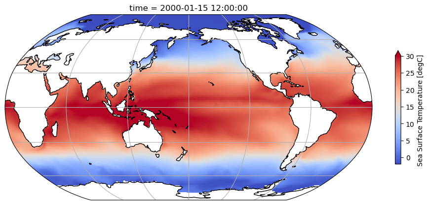
Visualize the first time slice to make sure the data looks okay
fig = plt.figure(figsize=(12, 6))
ax = plt.axes(projection=ccrs.Robinson(central_longitude=180))
ax.coastlines()
ax.gridlines()
ds.tos.isel(time=0).plot(
    ax=ax, transform=ccrs.PlateCarree(), vmin=-2, vmax=30, cbar_kwargs={'shrink': 0.5}, cmap='coolwarm'
);
Select the Niño 3.4 region
There are a couple ways we could selecting the Niño 3.4 region:
Use
sel()orisel()Use
where()and select all vlaues within the bounds of interest
1: sel:
tos_nino34 = ds.sel(lat=slice(-5, 5), lon=slice(190, 240))
tos_nino34
<xarray.Dataset>
Dimensions:    (time: 180, d2: 2, lat: 10, lon: 50)
Coordinates:
  * time       (time) object 2000-01-15 12:00:00 ... 2014-12-15 12:00:00
  * lat        (lat) float64 -4.5 -3.5 -2.5 -1.5 -0.5 0.5 1.5 2.5 3.5 4.5
  * lon        (lon) float64 190.5 191.5 192.5 193.5 ... 236.5 237.5 238.5 239.5
Dimensions without coordinates: d2
Data variables:
    time_bnds  (time, d2) object ...
    lat_bnds   (lat, d2) float64 ...
    lon_bnds   (lon, d2) float64 ...
    tos        (time, lat, lon) float32 ...
    areacello  (lat, lon) float64 ...
Attributes: (12/45)
    Conventions:            CF-1.7 CMIP-6.2
    activity_id:            CMIP
    branch_method:          standard
    branch_time_in_child:   674885.0
    branch_time_in_parent:  219000.0
    case_id:                972
    ...                     ...
    sub_experiment_id:      none
    table_id:               Omon
    tracking_id:            hdl:21.14100/2975ffd3-1d7b-47e3-961a-33f212ea4eb2
    variable_id:            tos
    variant_info:           CMIP6 20th century experiments (1850-2014) with C...
variant_label: r11i1p1f1- time: 180
- d2: 2
- lat: 10
- lon: 50
- time(time)object2000-01-15 12:00:00 ... 2014-12-...
- axis :
- T
- bounds :
- time_bnds
- standard_name :
- time
- title :
- time
- type :
- double
array([cftime.DatetimeNoLeap(2000, 1, 15, 12, 0, 0, 0, has_year_zero=True), cftime.DatetimeNoLeap(2000, 2, 14, 0, 0, 0, 0, has_year_zero=True), cftime.DatetimeNoLeap(2000, 3, 15, 12, 0, 0, 0, has_year_zero=True), cftime.DatetimeNoLeap(2000, 4, 15, 0, 0, 0, 0, has_year_zero=True), cftime.DatetimeNoLeap(2000, 5, 15, 12, 0, 0, 0, has_year_zero=True), cftime.DatetimeNoLeap(2000, 6, 15, 0, 0, 0, 0, has_year_zero=True), cftime.DatetimeNoLeap(2000, 7, 15, 12, 0, 0, 0, has_year_zero=True), cftime.DatetimeNoLeap(2000, 8, 15, 12, 0, 0, 0, has_year_zero=True), cftime.DatetimeNoLeap(2000, 9, 15, 0, 0, 0, 0, has_year_zero=True), cftime.DatetimeNoLeap(2000, 10, 15, 12, 0, 0, 0, has_year_zero=True), cftime.DatetimeNoLeap(2000, 11, 15, 0, 0, 0, 0, has_year_zero=True), cftime.DatetimeNoLeap(2000, 12, 15, 12, 0, 0, 0, has_year_zero=True), cftime.DatetimeNoLeap(2001, 1, 15, 12, 0, 0, 0, has_year_zero=True), cftime.DatetimeNoLeap(2001, 2, 14, 0, 0, 0, 0, has_year_zero=True), cftime.DatetimeNoLeap(2001, 3, 15, 12, 0, 0, 0, has_year_zero=True), cftime.DatetimeNoLeap(2001, 4, 15, 0, 0, 0, 0, has_year_zero=True), cftime.DatetimeNoLeap(2001, 5, 15, 12, 0, 0, 0, has_year_zero=True), cftime.DatetimeNoLeap(2001, 6, 15, 0, 0, 0, 0, has_year_zero=True), cftime.DatetimeNoLeap(2001, 7, 15, 12, 0, 0, 0, has_year_zero=True), cftime.DatetimeNoLeap(2001, 8, 15, 12, 0, 0, 0, has_year_zero=True), cftime.DatetimeNoLeap(2001, 9, 15, 0, 0, 0, 0, has_year_zero=True), cftime.DatetimeNoLeap(2001, 10, 15, 12, 0, 0, 0, has_year_zero=True), cftime.DatetimeNoLeap(2001, 11, 15, 0, 0, 0, 0, has_year_zero=True), cftime.DatetimeNoLeap(2001, 12, 15, 12, 0, 0, 0, has_year_zero=True), cftime.DatetimeNoLeap(2002, 1, 15, 12, 0, 0, 0, has_year_zero=True), cftime.DatetimeNoLeap(2002, 2, 14, 0, 0, 0, 0, has_year_zero=True), cftime.DatetimeNoLeap(2002, 3, 15, 12, 0, 0, 0, has_year_zero=True), cftime.DatetimeNoLeap(2002, 4, 15, 0, 0, 0, 0, has_year_zero=True), cftime.DatetimeNoLeap(2002, 5, 15, 12, 0, 0, 0, has_year_zero=True), cftime.DatetimeNoLeap(2002, 6, 15, 0, 0, 0, 0, has_year_zero=True), cftime.DatetimeNoLeap(2002, 7, 15, 12, 0, 0, 0, has_year_zero=True), cftime.DatetimeNoLeap(2002, 8, 15, 12, 0, 0, 0, has_year_zero=True), cftime.DatetimeNoLeap(2002, 9, 15, 0, 0, 0, 0, has_year_zero=True), cftime.DatetimeNoLeap(2002, 10, 15, 12, 0, 0, 0, has_year_zero=True), cftime.DatetimeNoLeap(2002, 11, 15, 0, 0, 0, 0, has_year_zero=True), cftime.DatetimeNoLeap(2002, 12, 15, 12, 0, 0, 0, has_year_zero=True), cftime.DatetimeNoLeap(2003, 1, 15, 12, 0, 0, 0, has_year_zero=True), cftime.DatetimeNoLeap(2003, 2, 14, 0, 0, 0, 0, has_year_zero=True), cftime.DatetimeNoLeap(2003, 3, 15, 12, 0, 0, 0, has_year_zero=True), cftime.DatetimeNoLeap(2003, 4, 15, 0, 0, 0, 0, has_year_zero=True), cftime.DatetimeNoLeap(2003, 5, 15, 12, 0, 0, 0, has_year_zero=True), cftime.DatetimeNoLeap(2003, 6, 15, 0, 0, 0, 0, has_year_zero=True), cftime.DatetimeNoLeap(2003, 7, 15, 12, 0, 0, 0, has_year_zero=True), cftime.DatetimeNoLeap(2003, 8, 15, 12, 0, 0, 0, has_year_zero=True), cftime.DatetimeNoLeap(2003, 9, 15, 0, 0, 0, 0, has_year_zero=True), cftime.DatetimeNoLeap(2003, 10, 15, 12, 0, 0, 0, has_year_zero=True), cftime.DatetimeNoLeap(2003, 11, 15, 0, 0, 0, 0, has_year_zero=True), cftime.DatetimeNoLeap(2003, 12, 15, 12, 0, 0, 0, has_year_zero=True), cftime.DatetimeNoLeap(2004, 1, 15, 12, 0, 0, 0, has_year_zero=True), cftime.DatetimeNoLeap(2004, 2, 14, 0, 0, 0, 0, has_year_zero=True), cftime.DatetimeNoLeap(2004, 3, 15, 12, 0, 0, 0, has_year_zero=True), cftime.DatetimeNoLeap(2004, 4, 15, 0, 0, 0, 0, has_year_zero=True), cftime.DatetimeNoLeap(2004, 5, 15, 12, 0, 0, 0, has_year_zero=True), cftime.DatetimeNoLeap(2004, 6, 15, 0, 0, 0, 0, has_year_zero=True), cftime.DatetimeNoLeap(2004, 7, 15, 12, 0, 0, 0, has_year_zero=True), cftime.DatetimeNoLeap(2004, 8, 15, 12, 0, 0, 0, has_year_zero=True), cftime.DatetimeNoLeap(2004, 9, 15, 0, 0, 0, 0, has_year_zero=True), cftime.DatetimeNoLeap(2004, 10, 15, 12, 0, 0, 0, has_year_zero=True), cftime.DatetimeNoLeap(2004, 11, 15, 0, 0, 0, 0, has_year_zero=True), cftime.DatetimeNoLeap(2004, 12, 15, 12, 0, 0, 0, has_year_zero=True), cftime.DatetimeNoLeap(2005, 1, 15, 12, 0, 0, 0, has_year_zero=True), cftime.DatetimeNoLeap(2005, 2, 14, 0, 0, 0, 0, has_year_zero=True), cftime.DatetimeNoLeap(2005, 3, 15, 12, 0, 0, 0, has_year_zero=True), cftime.DatetimeNoLeap(2005, 4, 15, 0, 0, 0, 0, has_year_zero=True), cftime.DatetimeNoLeap(2005, 5, 15, 12, 0, 0, 0, has_year_zero=True), cftime.DatetimeNoLeap(2005, 6, 15, 0, 0, 0, 0, has_year_zero=True), cftime.DatetimeNoLeap(2005, 7, 15, 12, 0, 0, 0, has_year_zero=True), cftime.DatetimeNoLeap(2005, 8, 15, 12, 0, 0, 0, has_year_zero=True), cftime.DatetimeNoLeap(2005, 9, 15, 0, 0, 0, 0, has_year_zero=True), cftime.DatetimeNoLeap(2005, 10, 15, 12, 0, 0, 0, has_year_zero=True), cftime.DatetimeNoLeap(2005, 11, 15, 0, 0, 0, 0, has_year_zero=True), cftime.DatetimeNoLeap(2005, 12, 15, 12, 0, 0, 0, has_year_zero=True), cftime.DatetimeNoLeap(2006, 1, 15, 12, 0, 0, 0, has_year_zero=True), cftime.DatetimeNoLeap(2006, 2, 14, 0, 0, 0, 0, has_year_zero=True), cftime.DatetimeNoLeap(2006, 3, 15, 12, 0, 0, 0, has_year_zero=True), cftime.DatetimeNoLeap(2006, 4, 15, 0, 0, 0, 0, has_year_zero=True), cftime.DatetimeNoLeap(2006, 5, 15, 12, 0, 0, 0, has_year_zero=True), cftime.DatetimeNoLeap(2006, 6, 15, 0, 0, 0, 0, has_year_zero=True), cftime.DatetimeNoLeap(2006, 7, 15, 12, 0, 0, 0, has_year_zero=True), cftime.DatetimeNoLeap(2006, 8, 15, 12, 0, 0, 0, has_year_zero=True), cftime.DatetimeNoLeap(2006, 9, 15, 0, 0, 0, 0, has_year_zero=True), cftime.DatetimeNoLeap(2006, 10, 15, 12, 0, 0, 0, has_year_zero=True), cftime.DatetimeNoLeap(2006, 11, 15, 0, 0, 0, 0, has_year_zero=True), cftime.DatetimeNoLeap(2006, 12, 15, 12, 0, 0, 0, has_year_zero=True), cftime.DatetimeNoLeap(2007, 1, 15, 12, 0, 0, 0, has_year_zero=True), cftime.DatetimeNoLeap(2007, 2, 14, 0, 0, 0, 0, has_year_zero=True), cftime.DatetimeNoLeap(2007, 3, 15, 12, 0, 0, 0, has_year_zero=True), cftime.DatetimeNoLeap(2007, 4, 15, 0, 0, 0, 0, has_year_zero=True), cftime.DatetimeNoLeap(2007, 5, 15, 12, 0, 0, 0, has_year_zero=True), cftime.DatetimeNoLeap(2007, 6, 15, 0, 0, 0, 0, has_year_zero=True), cftime.DatetimeNoLeap(2007, 7, 15, 12, 0, 0, 0, has_year_zero=True), cftime.DatetimeNoLeap(2007, 8, 15, 12, 0, 0, 0, has_year_zero=True), cftime.DatetimeNoLeap(2007, 9, 15, 0, 0, 0, 0, has_year_zero=True), cftime.DatetimeNoLeap(2007, 10, 15, 12, 0, 0, 0, has_year_zero=True), cftime.DatetimeNoLeap(2007, 11, 15, 0, 0, 0, 0, has_year_zero=True), cftime.DatetimeNoLeap(2007, 12, 15, 12, 0, 0, 0, has_year_zero=True), cftime.DatetimeNoLeap(2008, 1, 15, 12, 0, 0, 0, has_year_zero=True), cftime.DatetimeNoLeap(2008, 2, 14, 0, 0, 0, 0, has_year_zero=True), cftime.DatetimeNoLeap(2008, 3, 15, 12, 0, 0, 0, has_year_zero=True), cftime.DatetimeNoLeap(2008, 4, 15, 0, 0, 0, 0, has_year_zero=True), cftime.DatetimeNoLeap(2008, 5, 15, 12, 0, 0, 0, has_year_zero=True), cftime.DatetimeNoLeap(2008, 6, 15, 0, 0, 0, 0, has_year_zero=True), cftime.DatetimeNoLeap(2008, 7, 15, 12, 0, 0, 0, has_year_zero=True), cftime.DatetimeNoLeap(2008, 8, 15, 12, 0, 0, 0, has_year_zero=True), cftime.DatetimeNoLeap(2008, 9, 15, 0, 0, 0, 0, has_year_zero=True), cftime.DatetimeNoLeap(2008, 10, 15, 12, 0, 0, 0, has_year_zero=True), cftime.DatetimeNoLeap(2008, 11, 15, 0, 0, 0, 0, has_year_zero=True), cftime.DatetimeNoLeap(2008, 12, 15, 12, 0, 0, 0, has_year_zero=True), cftime.DatetimeNoLeap(2009, 1, 15, 12, 0, 0, 0, has_year_zero=True), cftime.DatetimeNoLeap(2009, 2, 14, 0, 0, 0, 0, has_year_zero=True), cftime.DatetimeNoLeap(2009, 3, 15, 12, 0, 0, 0, has_year_zero=True), cftime.DatetimeNoLeap(2009, 4, 15, 0, 0, 0, 0, has_year_zero=True), cftime.DatetimeNoLeap(2009, 5, 15, 12, 0, 0, 0, has_year_zero=True), cftime.DatetimeNoLeap(2009, 6, 15, 0, 0, 0, 0, has_year_zero=True), cftime.DatetimeNoLeap(2009, 7, 15, 12, 0, 0, 0, has_year_zero=True), cftime.DatetimeNoLeap(2009, 8, 15, 12, 0, 0, 0, has_year_zero=True), cftime.DatetimeNoLeap(2009, 9, 15, 0, 0, 0, 0, has_year_zero=True), cftime.DatetimeNoLeap(2009, 10, 15, 12, 0, 0, 0, has_year_zero=True), cftime.DatetimeNoLeap(2009, 11, 15, 0, 0, 0, 0, has_year_zero=True), cftime.DatetimeNoLeap(2009, 12, 15, 12, 0, 0, 0, has_year_zero=True), cftime.DatetimeNoLeap(2010, 1, 15, 12, 0, 0, 0, has_year_zero=True), cftime.DatetimeNoLeap(2010, 2, 14, 0, 0, 0, 0, has_year_zero=True), cftime.DatetimeNoLeap(2010, 3, 15, 12, 0, 0, 0, has_year_zero=True), cftime.DatetimeNoLeap(2010, 4, 15, 0, 0, 0, 0, has_year_zero=True), cftime.DatetimeNoLeap(2010, 5, 15, 12, 0, 0, 0, has_year_zero=True), cftime.DatetimeNoLeap(2010, 6, 15, 0, 0, 0, 0, has_year_zero=True), cftime.DatetimeNoLeap(2010, 7, 15, 12, 0, 0, 0, has_year_zero=True), cftime.DatetimeNoLeap(2010, 8, 15, 12, 0, 0, 0, has_year_zero=True), cftime.DatetimeNoLeap(2010, 9, 15, 0, 0, 0, 0, has_year_zero=True), cftime.DatetimeNoLeap(2010, 10, 15, 12, 0, 0, 0, has_year_zero=True), cftime.DatetimeNoLeap(2010, 11, 15, 0, 0, 0, 0, has_year_zero=True), cftime.DatetimeNoLeap(2010, 12, 15, 12, 0, 0, 0, has_year_zero=True), cftime.DatetimeNoLeap(2011, 1, 15, 12, 0, 0, 0, has_year_zero=True), cftime.DatetimeNoLeap(2011, 2, 14, 0, 0, 0, 0, has_year_zero=True), cftime.DatetimeNoLeap(2011, 3, 15, 12, 0, 0, 0, has_year_zero=True), cftime.DatetimeNoLeap(2011, 4, 15, 0, 0, 0, 0, has_year_zero=True), cftime.DatetimeNoLeap(2011, 5, 15, 12, 0, 0, 0, has_year_zero=True), cftime.DatetimeNoLeap(2011, 6, 15, 0, 0, 0, 0, has_year_zero=True), cftime.DatetimeNoLeap(2011, 7, 15, 12, 0, 0, 0, has_year_zero=True), cftime.DatetimeNoLeap(2011, 8, 15, 12, 0, 0, 0, has_year_zero=True), cftime.DatetimeNoLeap(2011, 9, 15, 0, 0, 0, 0, has_year_zero=True), cftime.DatetimeNoLeap(2011, 10, 15, 12, 0, 0, 0, has_year_zero=True), cftime.DatetimeNoLeap(2011, 11, 15, 0, 0, 0, 0, has_year_zero=True), cftime.DatetimeNoLeap(2011, 12, 15, 12, 0, 0, 0, has_year_zero=True), cftime.DatetimeNoLeap(2012, 1, 15, 12, 0, 0, 0, has_year_zero=True), cftime.DatetimeNoLeap(2012, 2, 14, 0, 0, 0, 0, has_year_zero=True), cftime.DatetimeNoLeap(2012, 3, 15, 12, 0, 0, 0, has_year_zero=True), cftime.DatetimeNoLeap(2012, 4, 15, 0, 0, 0, 0, has_year_zero=True), cftime.DatetimeNoLeap(2012, 5, 15, 12, 0, 0, 0, has_year_zero=True), cftime.DatetimeNoLeap(2012, 6, 15, 0, 0, 0, 0, has_year_zero=True), cftime.DatetimeNoLeap(2012, 7, 15, 12, 0, 0, 0, has_year_zero=True), cftime.DatetimeNoLeap(2012, 8, 15, 12, 0, 0, 0, has_year_zero=True), cftime.DatetimeNoLeap(2012, 9, 15, 0, 0, 0, 0, has_year_zero=True), cftime.DatetimeNoLeap(2012, 10, 15, 12, 0, 0, 0, has_year_zero=True), cftime.DatetimeNoLeap(2012, 11, 15, 0, 0, 0, 0, has_year_zero=True), cftime.DatetimeNoLeap(2012, 12, 15, 12, 0, 0, 0, has_year_zero=True), cftime.DatetimeNoLeap(2013, 1, 15, 12, 0, 0, 0, has_year_zero=True), cftime.DatetimeNoLeap(2013, 2, 14, 0, 0, 0, 0, has_year_zero=True), cftime.DatetimeNoLeap(2013, 3, 15, 12, 0, 0, 0, has_year_zero=True), cftime.DatetimeNoLeap(2013, 4, 15, 0, 0, 0, 0, has_year_zero=True), cftime.DatetimeNoLeap(2013, 5, 15, 12, 0, 0, 0, has_year_zero=True), cftime.DatetimeNoLeap(2013, 6, 15, 0, 0, 0, 0, has_year_zero=True), cftime.DatetimeNoLeap(2013, 7, 15, 12, 0, 0, 0, has_year_zero=True), cftime.DatetimeNoLeap(2013, 8, 15, 12, 0, 0, 0, has_year_zero=True), cftime.DatetimeNoLeap(2013, 9, 15, 0, 0, 0, 0, has_year_zero=True), cftime.DatetimeNoLeap(2013, 10, 15, 12, 0, 0, 0, has_year_zero=True), cftime.DatetimeNoLeap(2013, 11, 15, 0, 0, 0, 0, has_year_zero=True), cftime.DatetimeNoLeap(2013, 12, 15, 12, 0, 0, 0, has_year_zero=True), cftime.DatetimeNoLeap(2014, 1, 15, 12, 0, 0, 0, has_year_zero=True), cftime.DatetimeNoLeap(2014, 2, 14, 0, 0, 0, 0, has_year_zero=True), cftime.DatetimeNoLeap(2014, 3, 15, 12, 0, 0, 0, has_year_zero=True), cftime.DatetimeNoLeap(2014, 4, 15, 0, 0, 0, 0, has_year_zero=True), cftime.DatetimeNoLeap(2014, 5, 15, 12, 0, 0, 0, has_year_zero=True), cftime.DatetimeNoLeap(2014, 6, 15, 0, 0, 0, 0, has_year_zero=True), cftime.DatetimeNoLeap(2014, 7, 15, 12, 0, 0, 0, has_year_zero=True), cftime.DatetimeNoLeap(2014, 8, 15, 12, 0, 0, 0, has_year_zero=True), cftime.DatetimeNoLeap(2014, 9, 15, 0, 0, 0, 0, has_year_zero=True), cftime.DatetimeNoLeap(2014, 10, 15, 12, 0, 0, 0, has_year_zero=True), cftime.DatetimeNoLeap(2014, 11, 15, 0, 0, 0, 0, has_year_zero=True), cftime.DatetimeNoLeap(2014, 12, 15, 12, 0, 0, 0, has_year_zero=True)], dtype=object) - lat(lat)float64-4.5 -3.5 -2.5 -1.5 ... 2.5 3.5 4.5
- axis :
- Y
- bounds :
- lat_bnds
- long_name :
- latitude
- standard_name :
- latitude
- units :
- degrees_north
array([-4.5, -3.5, -2.5, -1.5, -0.5, 0.5, 1.5, 2.5, 3.5, 4.5])
- lon(lon)float64190.5 191.5 192.5 ... 238.5 239.5
- axis :
- X
- bounds :
- lon_bnds
- long_name :
- longitude
- standard_name :
- longitude
- units :
- degrees_east
array([190.5, 191.5, 192.5, 193.5, 194.5, 195.5, 196.5, 197.5, 198.5, 199.5,
       200.5, 201.5, 202.5, 203.5, 204.5, 205.5, 206.5, 207.5, 208.5, 209.5,
       210.5, 211.5, 212.5, 213.5, 214.5, 215.5, 216.5, 217.5, 218.5, 219.5,
       220.5, 221.5, 222.5, 223.5, 224.5, 225.5, 226.5, 227.5, 228.5, 229.5,
       230.5, 231.5, 232.5, 233.5, 234.5, 235.5, 236.5, 237.5, 238.5, 239.5])
- time_bnds(time, d2)object...
[360 values with dtype=object]
- lat_bnds(lat, d2)float64...
- long_name :
- latitude bounds
- units :
- degrees_north
[20 values with dtype=float64]
- lon_bnds(lon, d2)float64...
- long_name :
- longitude bounds
- units :
- degrees_east
[100 values with dtype=float64]
- tos(time, lat, lon)float32...
- cell_measures :
- area: areacello
- cell_methods :
- area: mean where sea time: mean
- comment :
- Model data on the 1x1 grid includes values in all cells for which ocean cells on the native grid cover more than 52.5 percent of the 1x1 grid cell. This 52.5 percent cutoff was chosen to produce ocean surface area on the 1x1 grid as close as possible to ocean surface area on the native grid, while not introducing fractional cell coverage.
- description :
- This may differ from "surface temperature" in regions of sea ice or floating ice shelves. For models using conservative temperature as the prognostic field, they should report the top ocean layer as surface potential temperature, which is the same as surface in situ temperature.
- frequency :
- mon
- id :
- tos
- long_name :
- Sea Surface Temperature
- mipTable :
- Omon
- out_name :
- tos
- prov :
- Omon ((isd.003))
- realm :
- ocean
- standard_name :
- sea_surface_temperature
- time :
- time
- time_label :
- time-mean
- time_title :
- Temporal mean
- title :
- Sea Surface Temperature
- type :
- real
- units :
- degC
- variable_id :
- tos
[90000 values with dtype=float32]
- areacello(lat, lon)float64...
- cell_methods :
- area: sum
- comment :
- TAREA
- description :
- Cell areas for any grid used to report ocean variables and variables which are requested as used on the model ocean grid (e.g. hfsso, which is a downward heat flux from the atmosphere interpolated onto the ocean grid). These cell areas should be defined to enable exact calculation of global integrals (e.g., of vertical fluxes of energy at the surface and top of the atmosphere).
- frequency :
- fx
- id :
- areacello
- long_name :
- Grid-Cell Area for Ocean Variables
- mipTable :
- Ofx
- out_name :
- areacello
- prov :
- Ofx ((isd.003))
- realm :
- ocean
- standard_name :
- cell_area
- time_label :
- None
- time_title :
- No temporal dimensions ... fixed field
- title :
- Grid-Cell Area for Ocean Variables
- type :
- real
- units :
- m2
- variable_id :
- areacello
[500 values with dtype=float64]
- timePandasIndex
PandasIndex(CFTimeIndex([2000-01-15 12:00:00, 2000-02-14 00:00:00, 2000-03-15 12:00:00, 2000-04-15 00:00:00, 2000-05-15 12:00:00, 2000-06-15 00:00:00, 2000-07-15 12:00:00, 2000-08-15 12:00:00, 2000-09-15 00:00:00, 2000-10-15 12:00:00, ... 2014-03-15 12:00:00, 2014-04-15 00:00:00, 2014-05-15 12:00:00, 2014-06-15 00:00:00, 2014-07-15 12:00:00, 2014-08-15 12:00:00, 2014-09-15 00:00:00, 2014-10-15 12:00:00, 2014-11-15 00:00:00, 2014-12-15 12:00:00], dtype='object', length=180, calendar='noleap', freq='None')) - latPandasIndex
PandasIndex(Index([-4.5, -3.5, -2.5, -1.5, -0.5, 0.5, 1.5, 2.5, 3.5, 4.5], dtype='float64', name='lat'))
- lonPandasIndex
PandasIndex(Index([190.5, 191.5, 192.5, 193.5, 194.5, 195.5, 196.5, 197.5, 198.5, 199.5,
       200.5, 201.5, 202.5, 203.5, 204.5, 205.5, 206.5, 207.5, 208.5, 209.5,
       210.5, 211.5, 212.5, 213.5, 214.5, 215.5, 216.5, 217.5, 218.5, 219.5,
       220.5, 221.5, 222.5, 223.5, 224.5, 225.5, 226.5, 227.5, 228.5, 229.5,
       230.5, 231.5, 232.5, 233.5, 234.5, 235.5, 236.5, 237.5, 238.5, 239.5],
      dtype='float64', name='lon'))
- Conventions :
- CF-1.7 CMIP-6.2
- activity_id :
- CMIP
- branch_method :
- standard
- branch_time_in_child :
- 674885.0
- branch_time_in_parent :
- 219000.0
- case_id :
- 972
- cesm_casename :
- b.e21.BHIST.f09_g17.CMIP6-historical.011
- contact :
- cesm_cmip6@ucar.edu
- creation_date :
- 2019-04-02T04:44:58Z
- data_specs_version :
- 01.00.29
- experiment :
- Simulation of recent past (1850 to 2014). Impose changing conditions (consistent with observations). Should be initialised from a point early enough in the pre-industrial control run to ensure that the end of all the perturbed runs branching from the end of this historical run end before the end of the control. Only one ensemble member is requested but modelling groups are strongly encouraged to submit at least three ensemble members of their CMIP historical simulation.
- experiment_id :
- historical
- external_variables :
- areacello
- forcing_index :
- 1
- frequency :
- mon
- further_info_url :
- https://furtherinfo.es-doc.org/CMIP6.NCAR.CESM2.historical.none.r11i1p1f1
- grid :
- ocean data regridded from native gx1v7 displaced pole grid (384x320 latxlon) to 180x360 latxlon using conservative regridding
- grid_label :
- gr
- initialization_index :
- 1
- institution :
- National Center for Atmospheric Research, Climate and Global Dynamics Laboratory, 1850 Table Mesa Drive, Boulder, CO 80305, USA
- institution_id :
- NCAR
- license :
- CMIP6 model data produced by <The National Center for Atmospheric Research> is licensed under a Creative Commons Attribution-[]ShareAlike 4.0 International License (https://creativecommons.org/licenses/). Consult https://pcmdi.llnl.gov/CMIP6/TermsOfUse for terms of use governing CMIP6 output, including citation requirements and proper acknowledgment. Further information about this data, including some limitations, can be found via the further_info_url (recorded as a global attribute in this file)[]. The data producers and data providers make no warranty, either express or implied, including, but not limited to, warranties of merchantability and fitness for a particular purpose. All liabilities arising from the supply of the information (including any liability arising in negligence) are excluded to the fullest extent permitted by law.
- mip_era :
- CMIP6
- model_doi_url :
- https://doi.org/10.5065/D67H1H0V
- nominal_resolution :
- 1x1 degree
- parent_activity_id :
- CMIP
- parent_experiment_id :
- piControl
- parent_mip_era :
- CMIP6
- parent_source_id :
- CESM2
- parent_time_units :
- days since 0001-01-01 00:00:00
- parent_variant_label :
- r1i1p1f1
- physics_index :
- 1
- product :
- model-output
- realization_index :
- 11
- realm :
- ocean
- source :
- CESM2 (2017): atmosphere: CAM6 (0.9x1.25 finite volume grid; 288 x 192 longitude/latitude; 32 levels; top level 2.25 mb); ocean: POP2 (320x384 longitude/latitude; 60 levels; top grid cell 0-10 m); sea_ice: CICE5.1 (same grid as ocean); land: CLM5 0.9x1.25 finite volume grid; 288 x 192 longitude/latitude; 32 levels; top level 2.25 mb); aerosol: MAM4 (0.9x1.25 finite volume grid; 288 x 192 longitude/latitude; 32 levels; top level 2.25 mb); atmoschem: MAM4 (0.9x1.25 finite volume grid; 288 x 192 longitude/latitude; 32 levels; top level 2.25 mb); landIce: CISM2.1; ocnBgchem: MARBL (320x384 longitude/latitude; 60 levels; top grid cell 0-10 m)
- source_id :
- CESM2
- source_type :
- AOGCM BGC
- sub_experiment :
- none
- sub_experiment_id :
- none
- table_id :
- Omon
- tracking_id :
- hdl:21.14100/2975ffd3-1d7b-47e3-961a-33f212ea4eb2
- variable_id :
- tos
- variant_info :
- CMIP6 20th century experiments (1850-2014) with CAM6, interactive land (CLM5), coupled ocean (POP2) with biogeochemistry (MARBL), interactive sea ice (CICE5.1), and non-evolving land ice (CISM2.1)
- variant_label :
- r11i1p1f1
2: where:
tos_nino34 = ds.where((ds.lat<5) & (ds.lat>-5) & (ds.lon>190) & (ds.lon<240), drop=True)
tos_nino34
<xarray.Dataset>
Dimensions:    (time: 180, d2: 2, lat: 10, lon: 50)
Coordinates:
  * time       (time) object 2000-01-15 12:00:00 ... 2014-12-15 12:00:00
  * lat        (lat) float64 -4.5 -3.5 -2.5 -1.5 -0.5 0.5 1.5 2.5 3.5 4.5
  * lon        (lon) float64 190.5 191.5 192.5 193.5 ... 236.5 237.5 238.5 239.5
Dimensions without coordinates: d2
Data variables:
    time_bnds  (time, d2, lat, lon) object 2000-01-01 00:00:00 ... 2015-01-01...
    lat_bnds   (lat, d2, lon) float64 -5.0 -5.0 -5.0 -5.0 ... 5.0 5.0 5.0 5.0
    lon_bnds   (lon, d2, lat) float64 190.0 190.0 190.0 ... 240.0 240.0 240.0
    tos        (time, lat, lon) float32 28.26 28.16 28.06 ... 28.54 28.57 28.63
    areacello  (lat, lon) float64 1.233e+10 1.233e+10 ... 1.233e+10 1.233e+10
Attributes: (12/45)
    Conventions:            CF-1.7 CMIP-6.2
    activity_id:            CMIP
    branch_method:          standard
    branch_time_in_child:   674885.0
    branch_time_in_parent:  219000.0
    case_id:                972
    ...                     ...
    sub_experiment_id:      none
    table_id:               Omon
    tracking_id:            hdl:21.14100/2975ffd3-1d7b-47e3-961a-33f212ea4eb2
    variable_id:            tos
    variant_info:           CMIP6 20th century experiments (1850-2014) with C...
variant_label: r11i1p1f1- time: 180
- d2: 2
- lat: 10
- lon: 50
- time(time)object2000-01-15 12:00:00 ... 2014-12-...
- axis :
- T
- bounds :
- time_bnds
- standard_name :
- time
- title :
- time
- type :
- double
array([cftime.DatetimeNoLeap(2000, 1, 15, 12, 0, 0, 0, has_year_zero=True), cftime.DatetimeNoLeap(2000, 2, 14, 0, 0, 0, 0, has_year_zero=True), cftime.DatetimeNoLeap(2000, 3, 15, 12, 0, 0, 0, has_year_zero=True), cftime.DatetimeNoLeap(2000, 4, 15, 0, 0, 0, 0, has_year_zero=True), cftime.DatetimeNoLeap(2000, 5, 15, 12, 0, 0, 0, has_year_zero=True), cftime.DatetimeNoLeap(2000, 6, 15, 0, 0, 0, 0, has_year_zero=True), cftime.DatetimeNoLeap(2000, 7, 15, 12, 0, 0, 0, has_year_zero=True), cftime.DatetimeNoLeap(2000, 8, 15, 12, 0, 0, 0, has_year_zero=True), cftime.DatetimeNoLeap(2000, 9, 15, 0, 0, 0, 0, has_year_zero=True), cftime.DatetimeNoLeap(2000, 10, 15, 12, 0, 0, 0, has_year_zero=True), cftime.DatetimeNoLeap(2000, 11, 15, 0, 0, 0, 0, has_year_zero=True), cftime.DatetimeNoLeap(2000, 12, 15, 12, 0, 0, 0, has_year_zero=True), cftime.DatetimeNoLeap(2001, 1, 15, 12, 0, 0, 0, has_year_zero=True), cftime.DatetimeNoLeap(2001, 2, 14, 0, 0, 0, 0, has_year_zero=True), cftime.DatetimeNoLeap(2001, 3, 15, 12, 0, 0, 0, has_year_zero=True), cftime.DatetimeNoLeap(2001, 4, 15, 0, 0, 0, 0, has_year_zero=True), cftime.DatetimeNoLeap(2001, 5, 15, 12, 0, 0, 0, has_year_zero=True), cftime.DatetimeNoLeap(2001, 6, 15, 0, 0, 0, 0, has_year_zero=True), cftime.DatetimeNoLeap(2001, 7, 15, 12, 0, 0, 0, has_year_zero=True), cftime.DatetimeNoLeap(2001, 8, 15, 12, 0, 0, 0, has_year_zero=True), cftime.DatetimeNoLeap(2001, 9, 15, 0, 0, 0, 0, has_year_zero=True), cftime.DatetimeNoLeap(2001, 10, 15, 12, 0, 0, 0, has_year_zero=True), cftime.DatetimeNoLeap(2001, 11, 15, 0, 0, 0, 0, has_year_zero=True), cftime.DatetimeNoLeap(2001, 12, 15, 12, 0, 0, 0, has_year_zero=True), cftime.DatetimeNoLeap(2002, 1, 15, 12, 0, 0, 0, has_year_zero=True), cftime.DatetimeNoLeap(2002, 2, 14, 0, 0, 0, 0, has_year_zero=True), cftime.DatetimeNoLeap(2002, 3, 15, 12, 0, 0, 0, has_year_zero=True), cftime.DatetimeNoLeap(2002, 4, 15, 0, 0, 0, 0, has_year_zero=True), cftime.DatetimeNoLeap(2002, 5, 15, 12, 0, 0, 0, has_year_zero=True), cftime.DatetimeNoLeap(2002, 6, 15, 0, 0, 0, 0, has_year_zero=True), cftime.DatetimeNoLeap(2002, 7, 15, 12, 0, 0, 0, has_year_zero=True), cftime.DatetimeNoLeap(2002, 8, 15, 12, 0, 0, 0, has_year_zero=True), cftime.DatetimeNoLeap(2002, 9, 15, 0, 0, 0, 0, has_year_zero=True), cftime.DatetimeNoLeap(2002, 10, 15, 12, 0, 0, 0, has_year_zero=True), cftime.DatetimeNoLeap(2002, 11, 15, 0, 0, 0, 0, has_year_zero=True), cftime.DatetimeNoLeap(2002, 12, 15, 12, 0, 0, 0, has_year_zero=True), cftime.DatetimeNoLeap(2003, 1, 15, 12, 0, 0, 0, has_year_zero=True), cftime.DatetimeNoLeap(2003, 2, 14, 0, 0, 0, 0, has_year_zero=True), cftime.DatetimeNoLeap(2003, 3, 15, 12, 0, 0, 0, has_year_zero=True), cftime.DatetimeNoLeap(2003, 4, 15, 0, 0, 0, 0, has_year_zero=True), cftime.DatetimeNoLeap(2003, 5, 15, 12, 0, 0, 0, has_year_zero=True), cftime.DatetimeNoLeap(2003, 6, 15, 0, 0, 0, 0, has_year_zero=True), cftime.DatetimeNoLeap(2003, 7, 15, 12, 0, 0, 0, has_year_zero=True), cftime.DatetimeNoLeap(2003, 8, 15, 12, 0, 0, 0, has_year_zero=True), cftime.DatetimeNoLeap(2003, 9, 15, 0, 0, 0, 0, has_year_zero=True), cftime.DatetimeNoLeap(2003, 10, 15, 12, 0, 0, 0, has_year_zero=True), cftime.DatetimeNoLeap(2003, 11, 15, 0, 0, 0, 0, has_year_zero=True), cftime.DatetimeNoLeap(2003, 12, 15, 12, 0, 0, 0, has_year_zero=True), cftime.DatetimeNoLeap(2004, 1, 15, 12, 0, 0, 0, has_year_zero=True), cftime.DatetimeNoLeap(2004, 2, 14, 0, 0, 0, 0, has_year_zero=True), cftime.DatetimeNoLeap(2004, 3, 15, 12, 0, 0, 0, has_year_zero=True), cftime.DatetimeNoLeap(2004, 4, 15, 0, 0, 0, 0, has_year_zero=True), cftime.DatetimeNoLeap(2004, 5, 15, 12, 0, 0, 0, has_year_zero=True), cftime.DatetimeNoLeap(2004, 6, 15, 0, 0, 0, 0, has_year_zero=True), cftime.DatetimeNoLeap(2004, 7, 15, 12, 0, 0, 0, has_year_zero=True), cftime.DatetimeNoLeap(2004, 8, 15, 12, 0, 0, 0, has_year_zero=True), cftime.DatetimeNoLeap(2004, 9, 15, 0, 0, 0, 0, has_year_zero=True), cftime.DatetimeNoLeap(2004, 10, 15, 12, 0, 0, 0, has_year_zero=True), cftime.DatetimeNoLeap(2004, 11, 15, 0, 0, 0, 0, has_year_zero=True), cftime.DatetimeNoLeap(2004, 12, 15, 12, 0, 0, 0, has_year_zero=True), cftime.DatetimeNoLeap(2005, 1, 15, 12, 0, 0, 0, has_year_zero=True), cftime.DatetimeNoLeap(2005, 2, 14, 0, 0, 0, 0, has_year_zero=True), cftime.DatetimeNoLeap(2005, 3, 15, 12, 0, 0, 0, has_year_zero=True), cftime.DatetimeNoLeap(2005, 4, 15, 0, 0, 0, 0, has_year_zero=True), cftime.DatetimeNoLeap(2005, 5, 15, 12, 0, 0, 0, has_year_zero=True), cftime.DatetimeNoLeap(2005, 6, 15, 0, 0, 0, 0, has_year_zero=True), cftime.DatetimeNoLeap(2005, 7, 15, 12, 0, 0, 0, has_year_zero=True), cftime.DatetimeNoLeap(2005, 8, 15, 12, 0, 0, 0, has_year_zero=True), cftime.DatetimeNoLeap(2005, 9, 15, 0, 0, 0, 0, has_year_zero=True), cftime.DatetimeNoLeap(2005, 10, 15, 12, 0, 0, 0, has_year_zero=True), cftime.DatetimeNoLeap(2005, 11, 15, 0, 0, 0, 0, has_year_zero=True), cftime.DatetimeNoLeap(2005, 12, 15, 12, 0, 0, 0, has_year_zero=True), cftime.DatetimeNoLeap(2006, 1, 15, 12, 0, 0, 0, has_year_zero=True), cftime.DatetimeNoLeap(2006, 2, 14, 0, 0, 0, 0, has_year_zero=True), cftime.DatetimeNoLeap(2006, 3, 15, 12, 0, 0, 0, has_year_zero=True), cftime.DatetimeNoLeap(2006, 4, 15, 0, 0, 0, 0, has_year_zero=True), cftime.DatetimeNoLeap(2006, 5, 15, 12, 0, 0, 0, has_year_zero=True), cftime.DatetimeNoLeap(2006, 6, 15, 0, 0, 0, 0, has_year_zero=True), cftime.DatetimeNoLeap(2006, 7, 15, 12, 0, 0, 0, has_year_zero=True), cftime.DatetimeNoLeap(2006, 8, 15, 12, 0, 0, 0, has_year_zero=True), cftime.DatetimeNoLeap(2006, 9, 15, 0, 0, 0, 0, has_year_zero=True), cftime.DatetimeNoLeap(2006, 10, 15, 12, 0, 0, 0, has_year_zero=True), cftime.DatetimeNoLeap(2006, 11, 15, 0, 0, 0, 0, has_year_zero=True), cftime.DatetimeNoLeap(2006, 12, 15, 12, 0, 0, 0, has_year_zero=True), cftime.DatetimeNoLeap(2007, 1, 15, 12, 0, 0, 0, has_year_zero=True), cftime.DatetimeNoLeap(2007, 2, 14, 0, 0, 0, 0, has_year_zero=True), cftime.DatetimeNoLeap(2007, 3, 15, 12, 0, 0, 0, has_year_zero=True), cftime.DatetimeNoLeap(2007, 4, 15, 0, 0, 0, 0, has_year_zero=True), cftime.DatetimeNoLeap(2007, 5, 15, 12, 0, 0, 0, has_year_zero=True), cftime.DatetimeNoLeap(2007, 6, 15, 0, 0, 0, 0, has_year_zero=True), cftime.DatetimeNoLeap(2007, 7, 15, 12, 0, 0, 0, has_year_zero=True), cftime.DatetimeNoLeap(2007, 8, 15, 12, 0, 0, 0, has_year_zero=True), cftime.DatetimeNoLeap(2007, 9, 15, 0, 0, 0, 0, has_year_zero=True), cftime.DatetimeNoLeap(2007, 10, 15, 12, 0, 0, 0, has_year_zero=True), cftime.DatetimeNoLeap(2007, 11, 15, 0, 0, 0, 0, has_year_zero=True), cftime.DatetimeNoLeap(2007, 12, 15, 12, 0, 0, 0, has_year_zero=True), cftime.DatetimeNoLeap(2008, 1, 15, 12, 0, 0, 0, has_year_zero=True), cftime.DatetimeNoLeap(2008, 2, 14, 0, 0, 0, 0, has_year_zero=True), cftime.DatetimeNoLeap(2008, 3, 15, 12, 0, 0, 0, has_year_zero=True), cftime.DatetimeNoLeap(2008, 4, 15, 0, 0, 0, 0, has_year_zero=True), cftime.DatetimeNoLeap(2008, 5, 15, 12, 0, 0, 0, has_year_zero=True), cftime.DatetimeNoLeap(2008, 6, 15, 0, 0, 0, 0, has_year_zero=True), cftime.DatetimeNoLeap(2008, 7, 15, 12, 0, 0, 0, has_year_zero=True), cftime.DatetimeNoLeap(2008, 8, 15, 12, 0, 0, 0, has_year_zero=True), cftime.DatetimeNoLeap(2008, 9, 15, 0, 0, 0, 0, has_year_zero=True), cftime.DatetimeNoLeap(2008, 10, 15, 12, 0, 0, 0, has_year_zero=True), cftime.DatetimeNoLeap(2008, 11, 15, 0, 0, 0, 0, has_year_zero=True), cftime.DatetimeNoLeap(2008, 12, 15, 12, 0, 0, 0, has_year_zero=True), cftime.DatetimeNoLeap(2009, 1, 15, 12, 0, 0, 0, has_year_zero=True), cftime.DatetimeNoLeap(2009, 2, 14, 0, 0, 0, 0, has_year_zero=True), cftime.DatetimeNoLeap(2009, 3, 15, 12, 0, 0, 0, has_year_zero=True), cftime.DatetimeNoLeap(2009, 4, 15, 0, 0, 0, 0, has_year_zero=True), cftime.DatetimeNoLeap(2009, 5, 15, 12, 0, 0, 0, has_year_zero=True), cftime.DatetimeNoLeap(2009, 6, 15, 0, 0, 0, 0, has_year_zero=True), cftime.DatetimeNoLeap(2009, 7, 15, 12, 0, 0, 0, has_year_zero=True), cftime.DatetimeNoLeap(2009, 8, 15, 12, 0, 0, 0, has_year_zero=True), cftime.DatetimeNoLeap(2009, 9, 15, 0, 0, 0, 0, has_year_zero=True), cftime.DatetimeNoLeap(2009, 10, 15, 12, 0, 0, 0, has_year_zero=True), cftime.DatetimeNoLeap(2009, 11, 15, 0, 0, 0, 0, has_year_zero=True), cftime.DatetimeNoLeap(2009, 12, 15, 12, 0, 0, 0, has_year_zero=True), cftime.DatetimeNoLeap(2010, 1, 15, 12, 0, 0, 0, has_year_zero=True), cftime.DatetimeNoLeap(2010, 2, 14, 0, 0, 0, 0, has_year_zero=True), cftime.DatetimeNoLeap(2010, 3, 15, 12, 0, 0, 0, has_year_zero=True), cftime.DatetimeNoLeap(2010, 4, 15, 0, 0, 0, 0, has_year_zero=True), cftime.DatetimeNoLeap(2010, 5, 15, 12, 0, 0, 0, has_year_zero=True), cftime.DatetimeNoLeap(2010, 6, 15, 0, 0, 0, 0, has_year_zero=True), cftime.DatetimeNoLeap(2010, 7, 15, 12, 0, 0, 0, has_year_zero=True), cftime.DatetimeNoLeap(2010, 8, 15, 12, 0, 0, 0, has_year_zero=True), cftime.DatetimeNoLeap(2010, 9, 15, 0, 0, 0, 0, has_year_zero=True), cftime.DatetimeNoLeap(2010, 10, 15, 12, 0, 0, 0, has_year_zero=True), cftime.DatetimeNoLeap(2010, 11, 15, 0, 0, 0, 0, has_year_zero=True), cftime.DatetimeNoLeap(2010, 12, 15, 12, 0, 0, 0, has_year_zero=True), cftime.DatetimeNoLeap(2011, 1, 15, 12, 0, 0, 0, has_year_zero=True), cftime.DatetimeNoLeap(2011, 2, 14, 0, 0, 0, 0, has_year_zero=True), cftime.DatetimeNoLeap(2011, 3, 15, 12, 0, 0, 0, has_year_zero=True), cftime.DatetimeNoLeap(2011, 4, 15, 0, 0, 0, 0, has_year_zero=True), cftime.DatetimeNoLeap(2011, 5, 15, 12, 0, 0, 0, has_year_zero=True), cftime.DatetimeNoLeap(2011, 6, 15, 0, 0, 0, 0, has_year_zero=True), cftime.DatetimeNoLeap(2011, 7, 15, 12, 0, 0, 0, has_year_zero=True), cftime.DatetimeNoLeap(2011, 8, 15, 12, 0, 0, 0, has_year_zero=True), cftime.DatetimeNoLeap(2011, 9, 15, 0, 0, 0, 0, has_year_zero=True), cftime.DatetimeNoLeap(2011, 10, 15, 12, 0, 0, 0, has_year_zero=True), cftime.DatetimeNoLeap(2011, 11, 15, 0, 0, 0, 0, has_year_zero=True), cftime.DatetimeNoLeap(2011, 12, 15, 12, 0, 0, 0, has_year_zero=True), cftime.DatetimeNoLeap(2012, 1, 15, 12, 0, 0, 0, has_year_zero=True), cftime.DatetimeNoLeap(2012, 2, 14, 0, 0, 0, 0, has_year_zero=True), cftime.DatetimeNoLeap(2012, 3, 15, 12, 0, 0, 0, has_year_zero=True), cftime.DatetimeNoLeap(2012, 4, 15, 0, 0, 0, 0, has_year_zero=True), cftime.DatetimeNoLeap(2012, 5, 15, 12, 0, 0, 0, has_year_zero=True), cftime.DatetimeNoLeap(2012, 6, 15, 0, 0, 0, 0, has_year_zero=True), cftime.DatetimeNoLeap(2012, 7, 15, 12, 0, 0, 0, has_year_zero=True), cftime.DatetimeNoLeap(2012, 8, 15, 12, 0, 0, 0, has_year_zero=True), cftime.DatetimeNoLeap(2012, 9, 15, 0, 0, 0, 0, has_year_zero=True), cftime.DatetimeNoLeap(2012, 10, 15, 12, 0, 0, 0, has_year_zero=True), cftime.DatetimeNoLeap(2012, 11, 15, 0, 0, 0, 0, has_year_zero=True), cftime.DatetimeNoLeap(2012, 12, 15, 12, 0, 0, 0, has_year_zero=True), cftime.DatetimeNoLeap(2013, 1, 15, 12, 0, 0, 0, has_year_zero=True), cftime.DatetimeNoLeap(2013, 2, 14, 0, 0, 0, 0, has_year_zero=True), cftime.DatetimeNoLeap(2013, 3, 15, 12, 0, 0, 0, has_year_zero=True), cftime.DatetimeNoLeap(2013, 4, 15, 0, 0, 0, 0, has_year_zero=True), cftime.DatetimeNoLeap(2013, 5, 15, 12, 0, 0, 0, has_year_zero=True), cftime.DatetimeNoLeap(2013, 6, 15, 0, 0, 0, 0, has_year_zero=True), cftime.DatetimeNoLeap(2013, 7, 15, 12, 0, 0, 0, has_year_zero=True), cftime.DatetimeNoLeap(2013, 8, 15, 12, 0, 0, 0, has_year_zero=True), cftime.DatetimeNoLeap(2013, 9, 15, 0, 0, 0, 0, has_year_zero=True), cftime.DatetimeNoLeap(2013, 10, 15, 12, 0, 0, 0, has_year_zero=True), cftime.DatetimeNoLeap(2013, 11, 15, 0, 0, 0, 0, has_year_zero=True), cftime.DatetimeNoLeap(2013, 12, 15, 12, 0, 0, 0, has_year_zero=True), cftime.DatetimeNoLeap(2014, 1, 15, 12, 0, 0, 0, has_year_zero=True), cftime.DatetimeNoLeap(2014, 2, 14, 0, 0, 0, 0, has_year_zero=True), cftime.DatetimeNoLeap(2014, 3, 15, 12, 0, 0, 0, has_year_zero=True), cftime.DatetimeNoLeap(2014, 4, 15, 0, 0, 0, 0, has_year_zero=True), cftime.DatetimeNoLeap(2014, 5, 15, 12, 0, 0, 0, has_year_zero=True), cftime.DatetimeNoLeap(2014, 6, 15, 0, 0, 0, 0, has_year_zero=True), cftime.DatetimeNoLeap(2014, 7, 15, 12, 0, 0, 0, has_year_zero=True), cftime.DatetimeNoLeap(2014, 8, 15, 12, 0, 0, 0, has_year_zero=True), cftime.DatetimeNoLeap(2014, 9, 15, 0, 0, 0, 0, has_year_zero=True), cftime.DatetimeNoLeap(2014, 10, 15, 12, 0, 0, 0, has_year_zero=True), cftime.DatetimeNoLeap(2014, 11, 15, 0, 0, 0, 0, has_year_zero=True), cftime.DatetimeNoLeap(2014, 12, 15, 12, 0, 0, 0, has_year_zero=True)], dtype=object) - lat(lat)float64-4.5 -3.5 -2.5 -1.5 ... 2.5 3.5 4.5
- axis :
- Y
- bounds :
- lat_bnds
- long_name :
- latitude
- standard_name :
- latitude
- units :
- degrees_north
array([-4.5, -3.5, -2.5, -1.5, -0.5, 0.5, 1.5, 2.5, 3.5, 4.5])
- lon(lon)float64190.5 191.5 192.5 ... 238.5 239.5
- axis :
- X
- bounds :
- lon_bnds
- long_name :
- longitude
- standard_name :
- longitude
- units :
- degrees_east
array([190.5, 191.5, 192.5, 193.5, 194.5, 195.5, 196.5, 197.5, 198.5, 199.5,
       200.5, 201.5, 202.5, 203.5, 204.5, 205.5, 206.5, 207.5, 208.5, 209.5,
       210.5, 211.5, 212.5, 213.5, 214.5, 215.5, 216.5, 217.5, 218.5, 219.5,
       220.5, 221.5, 222.5, 223.5, 224.5, 225.5, 226.5, 227.5, 228.5, 229.5,
       230.5, 231.5, 232.5, 233.5, 234.5, 235.5, 236.5, 237.5, 238.5, 239.5])
- time_bnds(time, d2, lat, lon)object2000-01-01 00:00:00 ... 2015-01-...
array([[[[cftime.DatetimeNoLeap(2000, 1, 1, 0, 0, 0, 0, has_year_zero=True), cftime.DatetimeNoLeap(2000, 1, 1, 0, 0, 0, 0, has_year_zero=True), cftime.DatetimeNoLeap(2000, 1, 1, 0, 0, 0, 0, has_year_zero=True), ..., cftime.DatetimeNoLeap(2000, 1, 1, 0, 0, 0, 0, has_year_zero=True), cftime.DatetimeNoLeap(2000, 1, 1, 0, 0, 0, 0, has_year_zero=True), cftime.DatetimeNoLeap(2000, 1, 1, 0, 0, 0, 0, has_year_zero=True)], [cftime.DatetimeNoLeap(2000, 1, 1, 0, 0, 0, 0, has_year_zero=True), cftime.DatetimeNoLeap(2000, 1, 1, 0, 0, 0, 0, has_year_zero=True), cftime.DatetimeNoLeap(2000, 1, 1, 0, 0, 0, 0, has_year_zero=True), ..., cftime.DatetimeNoLeap(2000, 1, 1, 0, 0, 0, 0, has_year_zero=True), cftime.DatetimeNoLeap(2000, 1, 1, 0, 0, 0, 0, has_year_zero=True), cftime.DatetimeNoLeap(2000, 1, 1, 0, 0, 0, 0, has_year_zero=True)], [cftime.DatetimeNoLeap(2000, 1, 1, 0, 0, 0, 0, has_year_zero=True), cftime.DatetimeNoLeap(2000, 1, 1, 0, 0, 0, 0, has_year_zero=True), cftime.DatetimeNoLeap(2000, 1, 1, 0, 0, 0, 0, has_year_zero=True), ..., cftime.DatetimeNoLeap(2000, 1, 1, 0, 0, 0, 0, has_year_zero=True), cftime.DatetimeNoLeap(2000, 1, 1, 0, 0, 0, 0, has_year_zero=True), ... cftime.DatetimeNoLeap(2015, 1, 1, 0, 0, 0, 0, has_year_zero=True), ..., cftime.DatetimeNoLeap(2015, 1, 1, 0, 0, 0, 0, has_year_zero=True), cftime.DatetimeNoLeap(2015, 1, 1, 0, 0, 0, 0, has_year_zero=True), cftime.DatetimeNoLeap(2015, 1, 1, 0, 0, 0, 0, has_year_zero=True)], [cftime.DatetimeNoLeap(2015, 1, 1, 0, 0, 0, 0, has_year_zero=True), cftime.DatetimeNoLeap(2015, 1, 1, 0, 0, 0, 0, has_year_zero=True), cftime.DatetimeNoLeap(2015, 1, 1, 0, 0, 0, 0, has_year_zero=True), ..., cftime.DatetimeNoLeap(2015, 1, 1, 0, 0, 0, 0, has_year_zero=True), cftime.DatetimeNoLeap(2015, 1, 1, 0, 0, 0, 0, has_year_zero=True), cftime.DatetimeNoLeap(2015, 1, 1, 0, 0, 0, 0, has_year_zero=True)], [cftime.DatetimeNoLeap(2015, 1, 1, 0, 0, 0, 0, has_year_zero=True), cftime.DatetimeNoLeap(2015, 1, 1, 0, 0, 0, 0, has_year_zero=True), cftime.DatetimeNoLeap(2015, 1, 1, 0, 0, 0, 0, has_year_zero=True), ..., cftime.DatetimeNoLeap(2015, 1, 1, 0, 0, 0, 0, has_year_zero=True), cftime.DatetimeNoLeap(2015, 1, 1, 0, 0, 0, 0, has_year_zero=True), cftime.DatetimeNoLeap(2015, 1, 1, 0, 0, 0, 0, has_year_zero=True)]]]], dtype=object) - lat_bnds(lat, d2, lon)float64-5.0 -5.0 -5.0 -5.0 ... 5.0 5.0 5.0
- long_name :
- latitude bounds
- units :
- degrees_north
array([[[-5., -5., -5., -5., -5., -5., -5., -5., -5., -5., -5., -5., -5., -5., -5., -5., -5., -5., -5., -5., -5., -5., -5., -5., -5., -5., -5., -5., -5., -5., -5., -5., -5., -5., -5., -5., -5., -5., -5., -5., -5., -5., -5., -5., -5., -5., -5., -5., -5., -5.], [-4., -4., -4., -4., -4., -4., -4., -4., -4., -4., -4., -4., -4., -4., -4., -4., -4., -4., -4., -4., -4., -4., -4., -4., -4., -4., -4., -4., -4., -4., -4., -4., -4., -4., -4., -4., -4., -4., -4., -4., -4., -4., -4., -4., -4., -4., -4., -4., -4., -4.]], [[-4., -4., -4., -4., -4., -4., -4., -4., -4., -4., -4., -4., -4., -4., -4., -4., -4., -4., -4., -4., -4., -4., -4., -4., -4., -4., -4., -4., -4., -4., -4., -4., -4., -4., -4., -4., -4., -4., -4., -4., -4., -4., -4., -4., -4., -4., -4., -4., -4., -4.], [-3., -3., -3., -3., -3., -3., -3., -3., -3., -3., -3., -3., -3., -3., -3., -3., -3., -3., -3., -3., -3., -3., -3., -3., -3., -3., -3., -3., -3., -3., -3., -3., -3., -3., -3., -3., -3., -3., -3., -3., -3., -3., -3., -3., -3., -3., -3., -3., ... 3., 3., 3., 3., 3., 3., 3., 3., 3., 3., 3., 3., 3., 3., 3., 3., 3., 3., 3., 3., 3., 3., 3., 3., 3., 3., 3., 3., 3., 3., 3., 3., 3., 3., 3., 3., 3., 3.], [ 4., 4., 4., 4., 4., 4., 4., 4., 4., 4., 4., 4., 4., 4., 4., 4., 4., 4., 4., 4., 4., 4., 4., 4., 4., 4., 4., 4., 4., 4., 4., 4., 4., 4., 4., 4., 4., 4., 4., 4., 4., 4., 4., 4., 4., 4., 4., 4., 4., 4.]], [[ 4., 4., 4., 4., 4., 4., 4., 4., 4., 4., 4., 4., 4., 4., 4., 4., 4., 4., 4., 4., 4., 4., 4., 4., 4., 4., 4., 4., 4., 4., 4., 4., 4., 4., 4., 4., 4., 4., 4., 4., 4., 4., 4., 4., 4., 4., 4., 4., 4., 4.], [ 5., 5., 5., 5., 5., 5., 5., 5., 5., 5., 5., 5., 5., 5., 5., 5., 5., 5., 5., 5., 5., 5., 5., 5., 5., 5., 5., 5., 5., 5., 5., 5., 5., 5., 5., 5., 5., 5., 5., 5., 5., 5., 5., 5., 5., 5., 5., 5., 5., 5.]]]) - lon_bnds(lon, d2, lat)float64190.0 190.0 190.0 ... 240.0 240.0
- long_name :
- longitude bounds
- units :
- degrees_east
array([[[190., 190., 190., 190., 190., 190., 190., 190., 190., 190.], [191., 191., 191., 191., 191., 191., 191., 191., 191., 191.]], [[191., 191., 191., 191., 191., 191., 191., 191., 191., 191.], [192., 192., 192., 192., 192., 192., 192., 192., 192., 192.]], [[192., 192., 192., 192., 192., 192., 192., 192., 192., 192.], [193., 193., 193., 193., 193., 193., 193., 193., 193., 193.]], [[193., 193., 193., 193., 193., 193., 193., 193., 193., 193.], [194., 194., 194., 194., 194., 194., 194., 194., 194., 194.]], [[194., 194., 194., 194., 194., 194., 194., 194., 194., 194.], [195., 195., 195., 195., 195., 195., 195., 195., 195., 195.]], [[195., 195., 195., 195., 195., 195., 195., 195., 195., 195.], [196., 196., 196., 196., 196., 196., 196., 196., 196., 196.]], [[196., 196., 196., 196., 196., 196., 196., 196., 196., 196.], [197., 197., 197., 197., 197., 197., 197., 197., 197., 197.]], ... [[233., 233., 233., 233., 233., 233., 233., 233., 233., 233.], [234., 234., 234., 234., 234., 234., 234., 234., 234., 234.]], [[234., 234., 234., 234., 234., 234., 234., 234., 234., 234.], [235., 235., 235., 235., 235., 235., 235., 235., 235., 235.]], [[235., 235., 235., 235., 235., 235., 235., 235., 235., 235.], [236., 236., 236., 236., 236., 236., 236., 236., 236., 236.]], [[236., 236., 236., 236., 236., 236., 236., 236., 236., 236.], [237., 237., 237., 237., 237., 237., 237., 237., 237., 237.]], [[237., 237., 237., 237., 237., 237., 237., 237., 237., 237.], [238., 238., 238., 238., 238., 238., 238., 238., 238., 238.]], [[238., 238., 238., 238., 238., 238., 238., 238., 238., 238.], [239., 239., 239., 239., 239., 239., 239., 239., 239., 239.]], [[239., 239., 239., 239., 239., 239., 239., 239., 239., 239.], [240., 240., 240., 240., 240., 240., 240., 240., 240., 240.]]]) - tos(time, lat, lon)float3228.26 28.16 28.06 ... 28.57 28.63
- cell_measures :
- area: areacello
- cell_methods :
- area: mean where sea time: mean
- comment :
- Model data on the 1x1 grid includes values in all cells for which ocean cells on the native grid cover more than 52.5 percent of the 1x1 grid cell. This 52.5 percent cutoff was chosen to produce ocean surface area on the 1x1 grid as close as possible to ocean surface area on the native grid, while not introducing fractional cell coverage.
- description :
- This may differ from "surface temperature" in regions of sea ice or floating ice shelves. For models using conservative temperature as the prognostic field, they should report the top ocean layer as surface potential temperature, which is the same as surface in situ temperature.
- frequency :
- mon
- id :
- tos
- long_name :
- Sea Surface Temperature
- mipTable :
- Omon
- out_name :
- tos
- prov :
- Omon ((isd.003))
- realm :
- ocean
- standard_name :
- sea_surface_temperature
- time :
- time
- time_label :
- time-mean
- time_title :
- Temporal mean
- title :
- Sea Surface Temperature
- type :
- real
- units :
- degC
- variable_id :
- tos
array([[[28.256025, 28.15772 , 28.057854, ..., 25.77648 , 25.707312, 25.583513], [27.947252, 27.849726, 27.748089, ..., 25.461096, 25.447067, 25.423643], [27.604124, 27.518108, 27.423113, ..., 25.094604, 25.086039, 25.157152], ..., [27.053625, 26.940416, 26.840393, ..., 25.746756, 25.579597, 25.118896], [27.316456, 27.217098, 27.137907, ..., 26.38955 , 26.240423, 25.860712], [27.787766, 27.727234, 27.68722 , ..., 27.01865 , 27.059557, 27.066883]], [[28.22752 , 28.158993, 28.10271 , ..., 26.485212, 26.45709 , 26.41093 ], [27.723951, 27.64461 , 27.570702, ..., 26.337622, 26.346348, 26.344204], [27.212313, 27.136517, 27.067299, ..., 26.119303, 26.17158 , 26.17856 ], ... [29.014107, 28.9657 , 28.918253, ..., 27.160896, 27.242203, 27.042742], [29.253191, 29.214586, 29.205938, ..., 27.537773, 27.626368, 27.471653], [29.873777, 29.819756, 29.793085, ..., 28.265177, 28.25255 , 28.158524]], [[29.728104, 29.645485, 29.56212 , ..., 26.747778, 26.701273, 26.655407], [29.253344, 29.176163, 29.104733, ..., 26.627005, 26.582062, 26.522951], [28.82321 , 28.737165, 28.669386, ..., 26.450716, 26.425608, 26.367132], ..., [28.780058, 28.769499, 28.78821 , ..., 27.061314, 27.029993, 27.031322], [29.100246, 29.051643, 29.008482, ..., 27.678553, 27.685179, 27.702488], [29.583574, 29.560463, 29.518036, ..., 28.542961, 28.569714, 28.62616 ]]], dtype=float32) - areacello(lat, lon)float641.233e+10 1.233e+10 ... 1.233e+10
- cell_methods :
- area: sum
- comment :
- TAREA
- description :
- Cell areas for any grid used to report ocean variables and variables which are requested as used on the model ocean grid (e.g. hfsso, which is a downward heat flux from the atmosphere interpolated onto the ocean grid). These cell areas should be defined to enable exact calculation of global integrals (e.g., of vertical fluxes of energy at the surface and top of the atmosphere).
- frequency :
- fx
- id :
- areacello
- long_name :
- Grid-Cell Area for Ocean Variables
- mipTable :
- Ofx
- out_name :
- areacello
- prov :
- Ofx ((isd.003))
- realm :
- ocean
- standard_name :
- cell_area
- time_label :
- None
- time_title :
- No temporal dimensions ... fixed field
- title :
- Grid-Cell Area for Ocean Variables
- type :
- real
- units :
- m2
- variable_id :
- areacello
array([[1.23271986e+10, 1.23271986e+10, 1.23271986e+10, 1.23271986e+10,
        1.23271986e+10, 1.23271986e+10, 1.23271986e+10, 1.23271986e+10,
        1.23271986e+10, 1.23271986e+10, 1.23271986e+10, 1.23271986e+10,
        1.23271986e+10, 1.23271986e+10, 1.23271986e+10, 1.23271986e+10,
        1.23271986e+10, 1.23271986e+10, 1.23271986e+10, 1.23271986e+10,
        1.23271986e+10, 1.23271986e+10, 1.23271986e+10, 1.23271986e+10,
        1.23271986e+10, 1.23271986e+10, 1.23271986e+10, 1.23271986e+10,
        1.23271986e+10, 1.23271986e+10, 1.23271986e+10, 1.23271986e+10,
        1.23271986e+10, 1.23271986e+10, 1.23271986e+10, 1.23271986e+10,
        1.23271986e+10, 1.23271986e+10, 1.23271986e+10, 1.23271986e+10,
        1.23271986e+10, 1.23271986e+10, 1.23271986e+10, 1.23271986e+10,
        1.23271986e+10, 1.23271986e+10, 1.23271986e+10, 1.23271986e+10,
        1.23271986e+10, 1.23271986e+10],
       [1.23422552e+10, 1.23422552e+10, 1.23422552e+10, 1.23422552e+10,
        1.23422552e+10, 1.23422552e+10, 1.23422552e+10, 1.23422552e+10,
        1.23422552e+10, 1.23422552e+10, 1.23422552e+10, 1.23422552e+10,
        1.23422552e+10, 1.23422552e+10, 1.23422552e+10, 1.23422552e+10,
        1.23422552e+10, 1.23422552e+10, 1.23422552e+10, 1.23422552e+10,
        1.23422552e+10, 1.23422552e+10, 1.23422552e+10, 1.23422552e+10,
        1.23422552e+10, 1.23422552e+10, 1.23422552e+10, 1.23422552e+10,
...
        1.23422552e+10, 1.23422552e+10, 1.23422552e+10, 1.23422552e+10,
        1.23422552e+10, 1.23422552e+10, 1.23422552e+10, 1.23422552e+10,
        1.23422552e+10, 1.23422552e+10, 1.23422552e+10, 1.23422552e+10,
        1.23422552e+10, 1.23422552e+10, 1.23422552e+10, 1.23422552e+10,
        1.23422552e+10, 1.23422552e+10, 1.23422552e+10, 1.23422552e+10,
        1.23422552e+10, 1.23422552e+10, 1.23422552e+10, 1.23422552e+10,
        1.23422552e+10, 1.23422552e+10],
       [1.23271986e+10, 1.23271986e+10, 1.23271986e+10, 1.23271986e+10,
        1.23271986e+10, 1.23271986e+10, 1.23271986e+10, 1.23271986e+10,
        1.23271986e+10, 1.23271986e+10, 1.23271986e+10, 1.23271986e+10,
        1.23271986e+10, 1.23271986e+10, 1.23271986e+10, 1.23271986e+10,
        1.23271986e+10, 1.23271986e+10, 1.23271986e+10, 1.23271986e+10,
        1.23271986e+10, 1.23271986e+10, 1.23271986e+10, 1.23271986e+10,
        1.23271986e+10, 1.23271986e+10, 1.23271986e+10, 1.23271986e+10,
        1.23271986e+10, 1.23271986e+10, 1.23271986e+10, 1.23271986e+10,
        1.23271986e+10, 1.23271986e+10, 1.23271986e+10, 1.23271986e+10,
        1.23271986e+10, 1.23271986e+10, 1.23271986e+10, 1.23271986e+10,
        1.23271986e+10, 1.23271986e+10, 1.23271986e+10, 1.23271986e+10,
        1.23271986e+10, 1.23271986e+10, 1.23271986e+10, 1.23271986e+10,
        1.23271986e+10, 1.23271986e+10]])
- timePandasIndex
PandasIndex(CFTimeIndex([2000-01-15 12:00:00, 2000-02-14 00:00:00, 2000-03-15 12:00:00, 2000-04-15 00:00:00, 2000-05-15 12:00:00, 2000-06-15 00:00:00, 2000-07-15 12:00:00, 2000-08-15 12:00:00, 2000-09-15 00:00:00, 2000-10-15 12:00:00, ... 2014-03-15 12:00:00, 2014-04-15 00:00:00, 2014-05-15 12:00:00, 2014-06-15 00:00:00, 2014-07-15 12:00:00, 2014-08-15 12:00:00, 2014-09-15 00:00:00, 2014-10-15 12:00:00, 2014-11-15 00:00:00, 2014-12-15 12:00:00], dtype='object', length=180, calendar='noleap', freq='None')) - latPandasIndex
PandasIndex(Index([-4.5, -3.5, -2.5, -1.5, -0.5, 0.5, 1.5, 2.5, 3.5, 4.5], dtype='float64', name='lat'))
- lonPandasIndex
PandasIndex(Index([190.5, 191.5, 192.5, 193.5, 194.5, 195.5, 196.5, 197.5, 198.5, 199.5,
       200.5, 201.5, 202.5, 203.5, 204.5, 205.5, 206.5, 207.5, 208.5, 209.5,
       210.5, 211.5, 212.5, 213.5, 214.5, 215.5, 216.5, 217.5, 218.5, 219.5,
       220.5, 221.5, 222.5, 223.5, 224.5, 225.5, 226.5, 227.5, 228.5, 229.5,
       230.5, 231.5, 232.5, 233.5, 234.5, 235.5, 236.5, 237.5, 238.5, 239.5],
      dtype='float64', name='lon'))
- Conventions :
- CF-1.7 CMIP-6.2
- activity_id :
- CMIP
- branch_method :
- standard
- branch_time_in_child :
- 674885.0
- branch_time_in_parent :
- 219000.0
- case_id :
- 972
- cesm_casename :
- b.e21.BHIST.f09_g17.CMIP6-historical.011
- contact :
- cesm_cmip6@ucar.edu
- creation_date :
- 2019-04-02T04:44:58Z
- data_specs_version :
- 01.00.29
- experiment :
- Simulation of recent past (1850 to 2014). Impose changing conditions (consistent with observations). Should be initialised from a point early enough in the pre-industrial control run to ensure that the end of all the perturbed runs branching from the end of this historical run end before the end of the control. Only one ensemble member is requested but modelling groups are strongly encouraged to submit at least three ensemble members of their CMIP historical simulation.
- experiment_id :
- historical
- external_variables :
- areacello
- forcing_index :
- 1
- frequency :
- mon
- further_info_url :
- https://furtherinfo.es-doc.org/CMIP6.NCAR.CESM2.historical.none.r11i1p1f1
- grid :
- ocean data regridded from native gx1v7 displaced pole grid (384x320 latxlon) to 180x360 latxlon using conservative regridding
- grid_label :
- gr
- initialization_index :
- 1
- institution :
- National Center for Atmospheric Research, Climate and Global Dynamics Laboratory, 1850 Table Mesa Drive, Boulder, CO 80305, USA
- institution_id :
- NCAR
- license :
- CMIP6 model data produced by <The National Center for Atmospheric Research> is licensed under a Creative Commons Attribution-[]ShareAlike 4.0 International License (https://creativecommons.org/licenses/). Consult https://pcmdi.llnl.gov/CMIP6/TermsOfUse for terms of use governing CMIP6 output, including citation requirements and proper acknowledgment. Further information about this data, including some limitations, can be found via the further_info_url (recorded as a global attribute in this file)[]. The data producers and data providers make no warranty, either express or implied, including, but not limited to, warranties of merchantability and fitness for a particular purpose. All liabilities arising from the supply of the information (including any liability arising in negligence) are excluded to the fullest extent permitted by law.
- mip_era :
- CMIP6
- model_doi_url :
- https://doi.org/10.5065/D67H1H0V
- nominal_resolution :
- 1x1 degree
- parent_activity_id :
- CMIP
- parent_experiment_id :
- piControl
- parent_mip_era :
- CMIP6
- parent_source_id :
- CESM2
- parent_time_units :
- days since 0001-01-01 00:00:00
- parent_variant_label :
- r1i1p1f1
- physics_index :
- 1
- product :
- model-output
- realization_index :
- 11
- realm :
- ocean
- source :
- CESM2 (2017): atmosphere: CAM6 (0.9x1.25 finite volume grid; 288 x 192 longitude/latitude; 32 levels; top level 2.25 mb); ocean: POP2 (320x384 longitude/latitude; 60 levels; top grid cell 0-10 m); sea_ice: CICE5.1 (same grid as ocean); land: CLM5 0.9x1.25 finite volume grid; 288 x 192 longitude/latitude; 32 levels; top level 2.25 mb); aerosol: MAM4 (0.9x1.25 finite volume grid; 288 x 192 longitude/latitude; 32 levels; top level 2.25 mb); atmoschem: MAM4 (0.9x1.25 finite volume grid; 288 x 192 longitude/latitude; 32 levels; top level 2.25 mb); landIce: CISM2.1; ocnBgchem: MARBL (320x384 longitude/latitude; 60 levels; top grid cell 0-10 m)
- source_id :
- CESM2
- source_type :
- AOGCM BGC
- sub_experiment :
- none
- sub_experiment_id :
- none
- table_id :
- Omon
- tracking_id :
- hdl:21.14100/2975ffd3-1d7b-47e3-961a-33f212ea4eb2
- variable_id :
- tos
- variant_info :
- CMIP6 20th century experiments (1850-2014) with CAM6, interactive land (CLM5), coupled ocean (POP2) with biogeochemistry (MARBL), interactive sea ice (CICE5.1), and non-evolving land ice (CISM2.1)
- variant_label :
- r11i1p1f1
Let’s plot the selected region to make sure we are doing the right thing.
fig = plt.figure(figsize=(12, 6))
ax = plt.axes(projection=ccrs.Robinson(central_longitude=180))
ax.coastlines()
ax.gridlines()
tos_nino34.tos.isel(time=0).plot(
    ax=ax, transform=ccrs.PlateCarree(), cbar_kwargs={'shrink': 0.5}, vmin=-2, vmax=30, cmap='coolwarm'
)
ax.set_extent((120, 300, 10, -10))
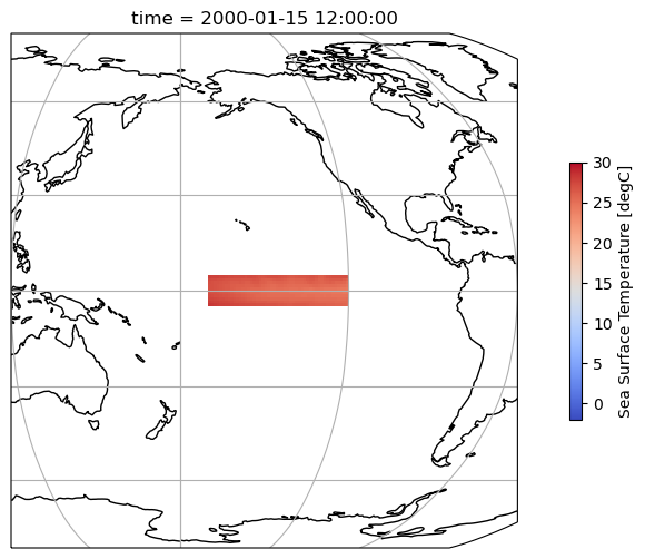
Compute monthly climatology
Compute the monthly climo for area averaged total SST from Niño 3.4 region, and subtract climatology from area averaged total SST time series to obtain anomalies
gb = tos_nino34.tos.groupby('time.month')
tos_nino34_anom = gb - gb.mean(dim='time')
index_nino34 = tos_nino34_anom.weighted(tos_nino34.areacello).mean(dim=['lat', 'lon'])
Smooth the anomalies with a 5-month running mean
index_nino34_rolling_mean = index_nino34.rolling(time=5,center=True).mean()
index_nino34.plot(size=8)
index_nino34_rolling_mean.plot()
plt.legend(['anomaly', '5-month running mean anomaly']);
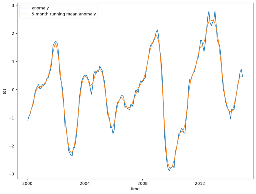
Normalize the smoothed values
We’ll normalize the values by dividing the rolling mean by the standard deviation.
std_dev = tos_nino34.tos.std()
std_dev
<xarray.DataArray 'tos' ()>
array(1.84363365)
- 1.844
array(1.84363365)
normalized_index_nino34_rolling_mean = index_nino34_rolling_mean / std_dev
Visualize the computed Niño 3.4 index.
We’ll highlight values in excess of 0.5, roughly corresponding to El Niño (warm) / La Niña (cold) events.
fig = plt.figure(figsize=(12, 6))

plt.fill_between(
    normalized_index_nino34_rolling_mean.time.data,
    normalized_index_nino34_rolling_mean.where(
        normalized_index_nino34_rolling_mean >= 0.4
    ).data,
    0.4,
    color='red',
    alpha=0.9,
)
plt.fill_between(
    normalized_index_nino34_rolling_mean.time.data,
    normalized_index_nino34_rolling_mean.where(
        normalized_index_nino34_rolling_mean <= -0.4
    ).data,
    -0.4,
    color='blue',
    alpha=0.9,
)

normalized_index_nino34_rolling_mean.plot(color='black')
plt.axhline(0, color='black', lw=0.5)
plt.axhline(0.4, color='black', linewidth=0.5, linestyle='dotted')
plt.axhline(-0.4, color='black', linewidth=0.5, linestyle='dotted')
plt.title('Niño 3.4 Index');
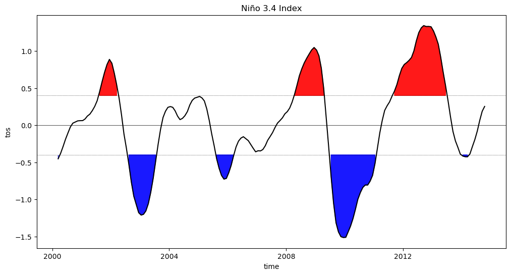
Summary
We have applied a variety of Xarray’s selection, grouping, and statistical functions to compute and visualize an important climate index.
What’s next?
In the next notebook, we will use Xarray to analyze and visualize NWP model output in another common format, GRIB.
Resources and References
Matplotlib’s
axhlinemethod (see also its analogousaxvlinemethod)