Shapefiles 2: Clip a raster within a shapefile
Contents
Shapefiles 2: Clip a raster within a shapefile
This notebook plots a raster (gridded) dataset and clips it to a vector shapefile.
Overview:
Use Xarray to read in a raster file; in this case, the most recent NCEP Real-time surface analysis (RTMA)
Use MetPy’s
parse_cfmethodRead in the Natural Earth state/province shapefile, georeferenced with Geopandas
Use Matplotlib and Cartopy methods to clip the raster field to fit exactly within the shapefile
Imports
import cartopy.crs as ccrs
import cartopy.feature as cfeature
from cartopy.mpl.patch import geos_to_path
import cartopy.io.shapereader as shpreader
from matplotlib import pyplot as plt
import matplotlib.path as mpath
import numpy as np
import xarray as xr
import os
from datetime import datetime, timedelta
os.environ['USE_PYGEOS'] = '0' # Eliminate warning message regarding PyGeos and Shapely with Geopandas
import geopandas as gpd
Select the regional bounds to subset the map (and, eventually, the data)
mapExtent = [-80,-71.3,40.2,45]
Specify the output map projection (Lambert Conformal, centered on New York State)
lon1 = -75
lat1 = 42.5
slat = 42.5

proj_map= ccrs.LambertConformal(central_longitude=lon1,
                             central_latitude=lat1,
                             standard_parallels=[slat,slat])
Access real-time NWP data from Unidata’s THREDDS server
Parse the current time and choose a recent hour when we might expect the model run to be complete. There is normally a ~90 minute lag, but we’ll give it a bit more than that.
now = datetime.now()
year = now.year
month = now.month
day = now.day
hour = now.hour
minute = now.minute
print (year, month, day, hour,minute)
2023 10 17 17 46
# The previous hour's data is typically available shortly after the half-hour, but give it a little extra time
if (minute < 45):
    hrDelta = 3
else:
    hrDelta = 2
runTime = now - timedelta(hours=hrDelta)
runTimeStr = runTime.strftime('%Y%m%d %H00 UTC')
modelDate = runTime.strftime('%Y%m%d')
modelHour = runTime.strftime('%H')
modelMin = runTime.strftime('%M')
modelDay = runTime.strftime('%D')
titleTime = modelDay + ' ' +  modelHour + '00 UTC'
print (modelDay)
print (modelHour)
print (runTimeStr)
print(titleTime)
10/17/23
15
20231017 1500 UTC
10/17/23 1500 UTC
runTime.strftime('%B')
'October'
Open the most recent NCEP real-time mesoscale analysis (RTMA) from Unidata’s THREDDS server
ds = xr.open_dataset(f'https://thredds.ucar.edu/thredds/dodsC/grib/NCEP/RTMA/CONUS_2p5km/RTMA_CONUS_2p5km_{modelDate}_{modelHour}00.grib2')
ds
<xarray.Dataset>
Dimensions:                                                              (
                                                                          x: 2145,
                                                                          y: 1377,
                                                                          time: 1,
                                                                          time1: 1,
                                                                          height_above_ground: 1,
                                                                          height_above_ground1: 1,
                                                                          altitude_above_msl: 1,
                                                                          time_bounds_1: 2)
Coordinates:
  * x                                                                    (x) float32 ...
  * y                                                                    (y) float32 ...
    reftime                                                              datetime64[ns] ...
  * time                                                                 (time) datetime64[ns] ...
  * time1                                                                (time1) datetime64[ns] ...
  * height_above_ground                                                  (height_above_ground) float32 ...
  * height_above_ground1                                                 (height_above_ground1) float32 ...
  * altitude_above_msl                                                   (altitude_above_msl) float32 ...
Dimensions without coordinates: time_bounds_1
Data variables: (12/22)
    LambertConformal_Projection                                          int32 ...
    time_bounds                                                          (time, time_bounds_1) datetime64[ns] ...
    Dewpoint_temperature_Analysis_height_above_ground                    (time1, height_above_ground1, y, x) float32 ...
    Dewpoint_temperature_error_height_above_ground                       (time1, height_above_ground1, y, x) float32 ...
    Geopotential_height_Analysis_surface                                 (time1, y, x) float32 ...
    Pressure_error_surface                                               (time1, y, x) float32 ...
    ...                                                                   ...
    Wind_speed_error_height_above_ground                                 (time1, height_above_ground, y, x) float32 ...
    Wind_speed_Analysis_height_above_ground                              (time1, height_above_ground, y, x) float32 ...
    Wind_speed_gust_Analysis_height_above_ground                         (time1, height_above_ground, y, x) float32 ...
    Wind_speed_gust_error_height_above_ground                            (time1, height_above_ground, y, x) float32 ...
    u-component_of_wind_Analysis_height_above_ground                     (time1, height_above_ground, y, x) float32 ...
    v-component_of_wind_Analysis_height_above_ground                     (time1, height_above_ground, y, x) float32 ...
Attributes:
    Originating_or_generating_Center:                                        ...
    Originating_or_generating_Subcenter:                                     ...
    GRIB_table_version:                                                      ...
    Type_of_generating_process:                                              ...
    Analysis_or_forecast_generating_process_identifier_defined_by_originating...
    file_format:                                                             ...
    Conventions:                                                             ...
    history:                                                                 ...
    featureType:                                                             ...
    _CoordSysBuilder:                                                        ...
EXTRA_DIMENSION.reftime: ...Leverage MetPy’s parse_cf function, which among other things will make it easy to extract the dataset’s map projection.
ds = ds.metpy.parse_cf()
ds
<xarray.Dataset>
Dimensions:                                                              (
                                                                          time: 1,
                                                                          time_bounds_1: 2,
                                                                          x: 2145,
                                                                          y: 1377,
                                                                          time1: 1,
                                                                          height_above_ground1: 1,
                                                                          altitude_above_msl: 1,
                                                                          height_above_ground: 1)
Coordinates:
    reftime                                                              datetime64[ns] ...
  * time                                                                 (time) datetime64[ns] ...
  * x                                                                    (x) float32 ...
  * y                                                                    (y) float32 ...
  * time1                                                                (time1) datetime64[ns] ...
  * height_above_ground1                                                 (height_above_ground1) float32 ...
    metpy_crs                                                            object ...
  * altitude_above_msl                                                   (altitude_above_msl) float32 ...
  * height_above_ground                                                  (height_above_ground) float32 ...
Dimensions without coordinates: time_bounds_1
Data variables: (12/22)
    LambertConformal_Projection                                          int32 ...
    time_bounds                                                          (time, time_bounds_1) datetime64[ns] ...
    Dewpoint_temperature_Analysis_height_above_ground                    (time1, height_above_ground1, y, x) float32 ...
    Dewpoint_temperature_error_height_above_ground                       (time1, height_above_ground1, y, x) float32 ...
    Geopotential_height_Analysis_surface                                 (time1, y, x) float32 ...
    Pressure_error_surface                                               (time1, y, x) float32 ...
    ...                                                                   ...
    Wind_speed_error_height_above_ground                                 (time1, height_above_ground, y, x) float32 ...
    Wind_speed_Analysis_height_above_ground                              (time1, height_above_ground, y, x) float32 ...
    Wind_speed_gust_Analysis_height_above_ground                         (time1, height_above_ground, y, x) float32 ...
    Wind_speed_gust_error_height_above_ground                            (time1, height_above_ground, y, x) float32 ...
    u-component_of_wind_Analysis_height_above_ground                     (time1, height_above_ground, y, x) float32 ...
    v-component_of_wind_Analysis_height_above_ground                     (time1, height_above_ground, y, x) float32 ...
Attributes:
    Originating_or_generating_Center:                                        ...
    Originating_or_generating_Subcenter:                                     ...
    GRIB_table_version:                                                      ...
    Type_of_generating_process:                                              ...
    Analysis_or_forecast_generating_process_identifier_defined_by_originating...
    file_format:                                                             ...
    Conventions:                                                             ...
    history:                                                                 ...
    featureType:                                                             ...
    _CoordSysBuilder:                                                        ...
EXTRA_DIMENSION.reftime: ...Note that there now exists a metpy_crs coordinate variable, which we’ll soon use to determine and use the Dataset’s map projection.
Select one of the variables from the Dataset; in this case, we’ll choose 2-meter temperature.
var = ds.Temperature_Analysis_height_above_ground
var
<xarray.DataArray 'Temperature_Analysis_height_above_ground' (time1: 1,
                                                              height_above_ground1: 1,
                                                              y: 1377, x: 2145)>
[2953665 values with dtype=float32]
Coordinates:
    reftime               datetime64[ns] 2023-10-17T15:00:00
  * x                     (x) float32 -2.763e+06 -2.761e+06 ... 2.682e+06
  * y                     (y) float32 -2.638e+05 -2.612e+05 ... 3.231e+06
  * time1                 (time1) datetime64[ns] 2023-10-17T15:00:00
  * height_above_ground1  (height_above_ground1) float32 2.0
    metpy_crs             object Projection: lambert_conformal_conic
Attributes: (12/13)
    long_name:                       Temperature Analysis @ Specified height ...
    units:                           K
    abbreviation:                    TMP
    grid_mapping:                    LambertConformal_Projection
    Grib_Variable_Id:                VAR_0-0-0_L103
    Grib2_Parameter:                 [0 0 0]
    ...                              ...
    Grib2_Parameter_Category:        Temperature
    Grib2_Parameter_Name:            Temperature
    Grib2_Level_Type:                103
    Grib2_Level_Desc:                Specified height level above ground
    Grib2_Generating_Process_Type:   Analysis
Grib2_Statistical_Process_Type: UnknownStatType--1Note that this DataArray has 3 dimensions; the time dimension has just one element. Let’s eliminate that time dimension using the .squeeze function.
var = var.squeeze()
var
<xarray.DataArray 'Temperature_Analysis_height_above_ground' (y: 1377, x: 2145)>
[2953665 values with dtype=float32]
Coordinates:
    reftime               datetime64[ns] 2023-10-17T15:00:00
  * x                     (x) float32 -2.763e+06 -2.761e+06 ... 2.682e+06
  * y                     (y) float32 -2.638e+05 -2.612e+05 ... 3.231e+06
    time1                 datetime64[ns] 2023-10-17T15:00:00
    height_above_ground1  float32 2.0
    metpy_crs             object Projection: lambert_conformal_conic
Attributes: (12/13)
    long_name:                       Temperature Analysis @ Specified height ...
    units:                           K
    abbreviation:                    TMP
    grid_mapping:                    LambertConformal_Projection
    Grib_Variable_Id:                VAR_0-0-0_L103
    Grib2_Parameter:                 [0 0 0]
    ...                              ...
    Grib2_Parameter_Category:        Temperature
    Grib2_Parameter_Name:            Temperature
    Grib2_Level_Type:                103
    Grib2_Level_Desc:                Specified height level above ground
    Grib2_Generating_Process_Type:   Analysis
Grib2_Statistical_Process_Type: UnknownStatType--1Now we can assign the Dataset’s map projection.
proj_data = var.metpy.cartopy_crs
proj_data
<cartopy.crs.LambertConformal object at 0x154f73c02c10>
Read in the 10m state/province shapefile
res = '10m'
category = 'cultural'
name = 'admin_1_states_provinces'
states = shpreader.natural_earth(res, category, name)
Read in the shapefile as a Geopandas dataframe
gdf = gpd.read_file(states)
Subset the Geopandas dataframe to just NYS and reset the index
gdf = gdf[gdf['name_en'] == 'New York'].reset_index(drop=True)
gdf
| featurecla | scalerank | adm1_code | diss_me | iso_3166_2 | wikipedia | iso_a2 | adm0_sr | name | name_alt | ... | name_nl | name_pl | name_pt | name_ru | name_sv | name_tr | name_vi | name_zh | ne_id | geometry | |
|---|---|---|---|---|---|---|---|---|---|---|---|---|---|---|---|---|---|---|---|---|---|
| 0 | Admin-1 scale rank | 2 | USA-3559 | 3559 | US-NY | http://en.wikipedia.org/wiki/New_York | US | 3 | New York | NY|N.Y. | ... | New York | Nowy Jork | Nova Iorque | Нью-Йорк | New York | New York | New York | 纽约州 | 1159312155 | MULTIPOLYGON (((-74.69588 44.99803, -74.59611 ... |
1 rows × 84 columns
Express the geometry in the desired map projection and create a new column for the output geometry
nystate_LCC = gdf.geometry.to_crs(proj_map)
gdf['geometryOutput'] = gdf.geometry.to_crs(proj_map)
gdf
| featurecla | scalerank | adm1_code | diss_me | iso_3166_2 | wikipedia | iso_a2 | adm0_sr | name | name_alt | ... | name_pl | name_pt | name_ru | name_sv | name_tr | name_vi | name_zh | ne_id | geometry | geometryOutput | |
|---|---|---|---|---|---|---|---|---|---|---|---|---|---|---|---|---|---|---|---|---|---|
| 0 | Admin-1 scale rank | 2 | USA-3559 | 3559 | US-NY | http://en.wikipedia.org/wiki/New_York | US | 3 | New York | NY|N.Y. | ... | Nowy Jork | Nova Iorque | Нью-Йорк | New York | New York | New York | 纽约州 | 1159312155 | MULTIPOLYGON (((-74.69588 44.99803, -74.59611 ... | MULTIPOLYGON (((24003.091 277681.072, 31876.47... |
1 rows × 85 columns
Express the output map projection geometry as a Matplotlib path. We pass in a Shapely geometry object from the first (and in this case, only) row to Cartopy’s geos_to_path function.
path = geos_to_path(gdf.loc[0,'geometryOutput'])
var
<xarray.DataArray 'Temperature_Analysis_height_above_ground' (y: 1377, x: 2145)>
[2953665 values with dtype=float32]
Coordinates:
    reftime               datetime64[ns] 2023-10-17T15:00:00
  * x                     (x) float32 -2.763e+06 -2.761e+06 ... 2.682e+06
  * y                     (y) float32 -2.638e+05 -2.612e+05 ... 3.231e+06
    time1                 datetime64[ns] 2023-10-17T15:00:00
    height_above_ground1  float32 2.0
    metpy_crs             object Projection: lambert_conformal_conic
Attributes: (12/13)
    long_name:                       Temperature Analysis @ Specified height ...
    units:                           K
    abbreviation:                    TMP
    grid_mapping:                    LambertConformal_Projection
    Grib_Variable_Id:                VAR_0-0-0_L103
    Grib2_Parameter:                 [0 0 0]
    ...                              ...
    Grib2_Parameter_Category:        Temperature
    Grib2_Parameter_Name:            Temperature
    Grib2_Level_Type:                103
    Grib2_Level_Desc:                Specified height level above ground
    Grib2_Generating_Process_Type:   Analysis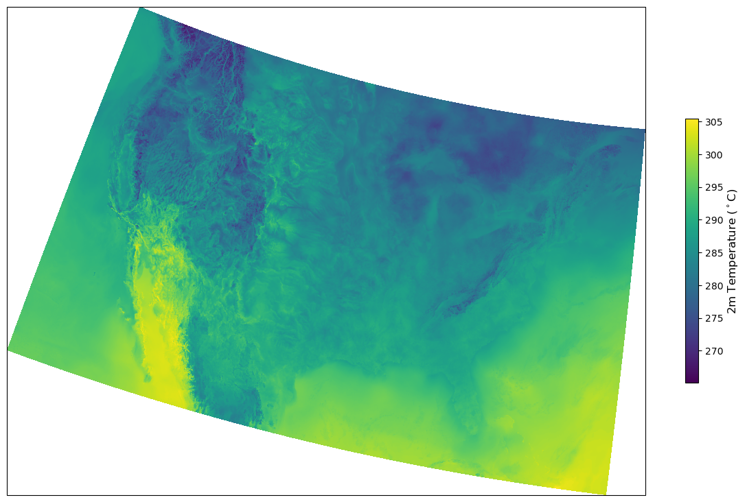
Grib2_Statistical_Process_Type: UnknownStatType--1fig, ax1 = plt.subplots(nrows=1, figsize=(15,10), subplot_kw={"projection": proj_map})
x, y = var.x, var.y
mesh = ax1.pcolormesh(x, y, var, transform=proj_data)
# Make a colorbar
cbar = fig.colorbar(mesh,shrink=0.5)
cbar.set_label(r'2m Temperature ($^\circ$C)', size='large')
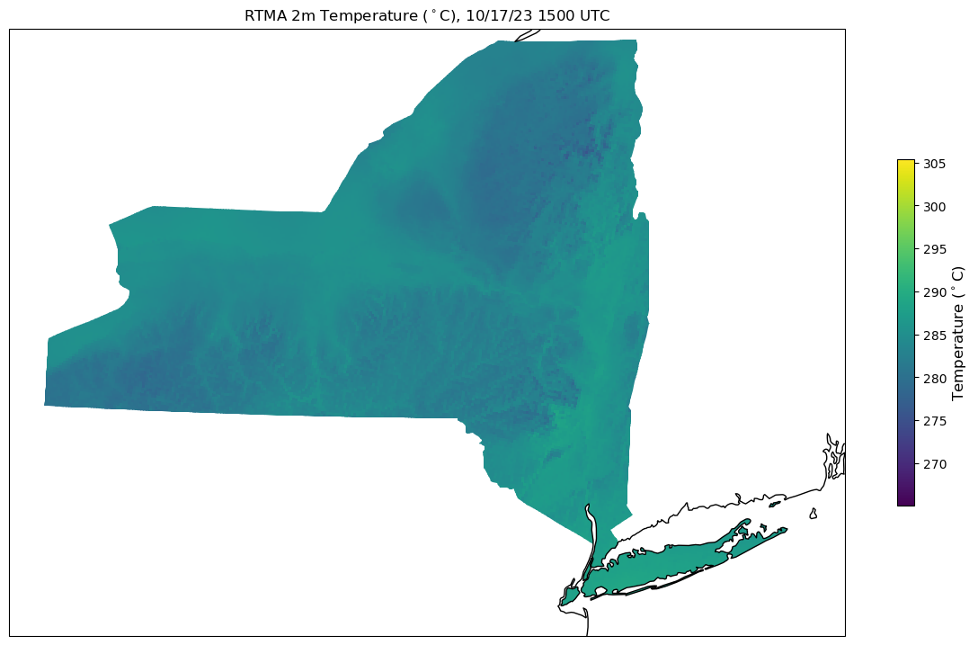
Now, let’s use some Matplotlib magic to clip the raster data so it only is displayed within the NYS 10m shapefile.
poly_path = path
poly_compound_path = mpath.Path.make_compound_path(*poly_path)
poly_transform = proj_map._as_mpl_transform(ax1)
mesh.set_clip_path(poly_compound_path, poly_transform)
res='10m'

fig, ax1 = plt.subplots(nrows=1, figsize=(15,10), subplot_kw={"projection": proj_map})

ax1.set_extent(mapExtent,crs=ccrs.PlateCarree())

mesh = ax1.pcolormesh(x, y, var, transform=proj_data)
# Make a colorbar
cbar = fig.colorbar(mesh,shrink=0.5)
cbar.set_label(f'Temperature ($^\circ$C)', size='large')
ax1.coastlines()

# Get the path of the polygons
#poly_path = nypath
poly_path = path
poly_compound_path = mpath.Path.make_compound_path(*poly_path)
poly_transform = proj_map._as_mpl_transform(ax1)
mesh.set_clip_path(poly_compound_path, poly_transform)
ax1.set_title(f'RTMA 2m Temperature ($^\circ$C), {titleTime}');
Things to try:
Overlay additional data (point-based, contour-based, etc.) on the final map
Use the data variable’s metadata to dynamically create the figure title and/or colorbar label.
When you create the Xarray dataset, use
selto restrict the spatial extent of the data retrieval.