Xarray 4: Remote access
Contents
Xarray 4: Remote access
Overview
Work with a multiple-file Xarray
Datasethosted on NCAR’s Research Data ArchiveSubset the Dataset along its dimensions
Perform unit conversion
Create a well-labeled multi-parameter contour plot of gridded ERA-5 reanalysis data
Imports
import xarray as xr
import pandas as pd
import numpy as np
from datetime import datetime as dt
from metpy.units import units
from metpy import calc as mpcalc
import cartopy.crs as ccrs
import cartopy.feature as cfeature
import matplotlib.pyplot as plt
import requests
from pathlib import Path
Work with the ERA-5 Dataset hosted on NCAR’s Remote Data Archive
Datasets are ever-growing in terms of size and sheer number. It is not “remotely” possible to download every dataset one might want to use to your computer! Fortunately, although Xarray provides easy access to files stored “locally” on disk, it can also give you access to files stored on remotely-located servers via different types of data access protocols. One such protocol is called OpenDAP. It makes files available via a specially-crafted web link, or URL. This is how we will access ERA-5 datasets stored on the ERA-5 RDA’s THREDDS server data catalog.
Construct OpenDAP URL’s for the ERA-5 datasets served by the RDA server.
ds_urlp = 'https://thredds.rda.ucar.edu/thredds/dodsC/files/g/ds633.0/e5.oper.an.sfc/201210/e5.oper.an.sfc.128_151_msl.ll025sc.2012100100_2012103123.nc'
ds_urlz = 'https://thredds.rda.ucar.edu/thredds/dodsC/files/g/ds633.0/e5.oper.an.pl/201210/e5.oper.an.pl.128_129_z.ll025sc.2012103000_2012103023.nc'
Now open the two files as separate Datasets. (avoid using open_mfdataset as subsetting will cause failures down the line)
open_mfdataset, that allows for one Dataset to be created from multiple sources. However, this may lead to strange errors after we subset the data later in this notebook. This problem seems specific to using open_mfdataset on file served by THREDDS.
dsSLP = xr.open_dataset(ds_urlp)
dsZ = xr.open_dataset(ds_urlz)
Let’s see what one of these Datasets looks like.
dsZ
<xarray.Dataset>
Dimensions:    (latitude: 721, level: 37, longitude: 1440, time: 24)
Coordinates:
  * latitude   (latitude) float64 90.0 89.75 89.5 89.25 ... -89.5 -89.75 -90.0
  * level      (level) float64 1.0 2.0 3.0 5.0 7.0 ... 925.0 950.0 975.0 1e+03
  * longitude  (longitude) float64 0.0 0.25 0.5 0.75 ... 359.0 359.2 359.5 359.8
  * time       (time) datetime64[ns] 2012-10-30 ... 2012-10-30T23:00:00
Data variables:
    utc_date   (time) int32 ...
    Z          (time, level, latitude, longitude) float32 ...
Attributes:
    _NCProperties:                   version=1|netcdflibversion=4.6.1|hdf5lib...
    DATA_SOURCE:                     ECMWF: https://cds.climate.copernicus.eu...
    NETCDF_CONVERSION:               CISL RDA: Conversion from ECMWF GRIB 1 d...
    NETCDF_VERSION:                  4.6.1
    CONVERSION_PLATFORM:             Linux casper21 3.10.0-693.21.1.el7.x86_6...
    CONVERSION_DATE:                 Mon Aug 26 17:48:10 MDT 2019
    Conventions:                     CF-1.6
    NETCDF_COMPRESSION:              NCO: Precision-preserving compression to...
    history:                         Mon Aug 26 17:48:45 2019: ncks -4 --ppc ...
    NCO:                             netCDF Operators version 4.7.4 (http://n...
DODS_EXTRA.Unlimited_Dimension: timedsSLP
<xarray.Dataset>
Dimensions:    (latitude: 721, longitude: 1440, time: 744)
Coordinates:
  * latitude   (latitude) float64 90.0 89.75 89.5 89.25 ... -89.5 -89.75 -90.0
  * longitude  (longitude) float64 0.0 0.25 0.5 0.75 ... 359.0 359.2 359.5 359.8
  * time       (time) datetime64[ns] 2012-10-01 ... 2012-10-31T23:00:00
Data variables:
    utc_date   (time) int32 ...
    MSL        (time, latitude, longitude) float32 ...
Attributes:
    _NCProperties:                   version=1|netcdflibversion=4.6.1|hdf5lib...
    DATA_SOURCE:                     ECMWF: https://cds.climate.copernicus.eu...
    NETCDF_CONVERSION:               CISL RDA: Conversion from ECMWF GRIB1 da...
    NETCDF_VERSION:                  4.6.1
    CONVERSION_PLATFORM:             Linux casper21 3.10.0-693.21.1.el7.x86_6...
    CONVERSION_DATE:                 Mon Aug 26 16:01:50 MDT 2019
    Conventions:                     CF-1.6
    NETCDF_COMPRESSION:              NCO: Precision-preserving compression to...
    history:                         Mon Aug 26 16:02:17 2019: ncks -4 --ppc ...
    NCO:                             netCDF Operators version 4.7.4 (http://n...
DODS_EXTRA.Unlimited_Dimension: timedsSize = dsZ.nbytes / 1e9
print ("Size of dataset = %.3f GB" % dsSize)
Size of dataset = 3.688 GB
Subset the Dataset along its dimensions
We noticed in the previous notebook that our contour labels were not appearing with every contour line. This is because we passed the entire horizontal extent (all latitudes and longitudes) to the ax.contour method. Since our intent is to plot only over a regional subset, we will use the sel method on the latitude and longitude dimensions as well as time and isobaric surface.
We’ll also use Datetime and string methods to more dynamically assign various dimensional specifications, as well as aid in figure-labeling later on.
# Areal extent
lonW = -100
lonE = -60
latS = 20
latN = 50
latRange = np.arange(latS-5,latN+5,.25) # expand the data range a bit beyond the plot range
lonRange = np.arange((lonW-5+360),(lonE+5+360),.25) # Need to match longitude values to those of the coordinate variable

# Vertical level specificaton
vlevel = 500
levelStr = str(vlevel)

# Date/Time specification
Year = 2012
Month = 10
Day = 30
Hour = 0
Minute = 0
dateTime = dt(Year,Month,Day, Hour, Minute)
timeStr = dateTime.strftime("%Y-%m-%d %H%M UTC")

# Data variable selection

SLP = dsSLP['MSL'].sel(time=dateTime,latitude=latRange,longitude=lonRange)
Z = dsZ['Z'].sel(time=dateTime,latitude=latRange,longitude=lonRange,level=vlevel)
Let’s look at some of the attributes
Z.shape
(160, 200)
Z.dims
('latitude', 'longitude')
Z.units
'm**2 s**-2'
SLP.shape
(160, 200)
SLP.dims
('latitude', 'longitude')
SLP.units
'Pa'
Define our subsetted coordinate arrays of lat and lon. Pull them from any of the DataArrays. We’ll need to pass these into the contouring functions later on.
lats = SLP.latitude
lons = SLP.longitude
lats
<xarray.DataArray 'latitude' (latitude: 160)>
array([15.  , 15.25, 15.5 , 15.75, 16.  , 16.25, 16.5 , 16.75, 17.  , 17.25,
       17.5 , 17.75, 18.  , 18.25, 18.5 , 18.75, 19.  , 19.25, 19.5 , 19.75,
       20.  , 20.25, 20.5 , 20.75, 21.  , 21.25, 21.5 , 21.75, 22.  , 22.25,
       22.5 , 22.75, 23.  , 23.25, 23.5 , 23.75, 24.  , 24.25, 24.5 , 24.75,
       25.  , 25.25, 25.5 , 25.75, 26.  , 26.25, 26.5 , 26.75, 27.  , 27.25,
       27.5 , 27.75, 28.  , 28.25, 28.5 , 28.75, 29.  , 29.25, 29.5 , 29.75,
       30.  , 30.25, 30.5 , 30.75, 31.  , 31.25, 31.5 , 31.75, 32.  , 32.25,
       32.5 , 32.75, 33.  , 33.25, 33.5 , 33.75, 34.  , 34.25, 34.5 , 34.75,
       35.  , 35.25, 35.5 , 35.75, 36.  , 36.25, 36.5 , 36.75, 37.  , 37.25,
       37.5 , 37.75, 38.  , 38.25, 38.5 , 38.75, 39.  , 39.25, 39.5 , 39.75,
       40.  , 40.25, 40.5 , 40.75, 41.  , 41.25, 41.5 , 41.75, 42.  , 42.25,
       42.5 , 42.75, 43.  , 43.25, 43.5 , 43.75, 44.  , 44.25, 44.5 , 44.75,
       45.  , 45.25, 45.5 , 45.75, 46.  , 46.25, 46.5 , 46.75, 47.  , 47.25,
       47.5 , 47.75, 48.  , 48.25, 48.5 , 48.75, 49.  , 49.25, 49.5 , 49.75,
       50.  , 50.25, 50.5 , 50.75, 51.  , 51.25, 51.5 , 51.75, 52.  , 52.25,
       52.5 , 52.75, 53.  , 53.25, 53.5 , 53.75, 54.  , 54.25, 54.5 , 54.75])
Coordinates:
  * latitude  (latitude) float64 15.0 15.25 15.5 15.75 ... 54.0 54.25 54.5 54.75
    time      datetime64[ns] 2012-10-30
Attributes:
    long_name:    latitude
    short_name:   lat
    units:        degrees_north
    qualifier:    Gaussian
_ChunkSizes: 721lons
<xarray.DataArray 'longitude' (longitude: 200)>
array([255.  , 255.25, 255.5 , 255.75, 256.  , 256.25, 256.5 , 256.75, 257.  ,
       257.25, 257.5 , 257.75, 258.  , 258.25, 258.5 , 258.75, 259.  , 259.25,
       259.5 , 259.75, 260.  , 260.25, 260.5 , 260.75, 261.  , 261.25, 261.5 ,
       261.75, 262.  , 262.25, 262.5 , 262.75, 263.  , 263.25, 263.5 , 263.75,
       264.  , 264.25, 264.5 , 264.75, 265.  , 265.25, 265.5 , 265.75, 266.  ,
       266.25, 266.5 , 266.75, 267.  , 267.25, 267.5 , 267.75, 268.  , 268.25,
       268.5 , 268.75, 269.  , 269.25, 269.5 , 269.75, 270.  , 270.25, 270.5 ,
       270.75, 271.  , 271.25, 271.5 , 271.75, 272.  , 272.25, 272.5 , 272.75,
       273.  , 273.25, 273.5 , 273.75, 274.  , 274.25, 274.5 , 274.75, 275.  ,
       275.25, 275.5 , 275.75, 276.  , 276.25, 276.5 , 276.75, 277.  , 277.25,
       277.5 , 277.75, 278.  , 278.25, 278.5 , 278.75, 279.  , 279.25, 279.5 ,
       279.75, 280.  , 280.25, 280.5 , 280.75, 281.  , 281.25, 281.5 , 281.75,
       282.  , 282.25, 282.5 , 282.75, 283.  , 283.25, 283.5 , 283.75, 284.  ,
       284.25, 284.5 , 284.75, 285.  , 285.25, 285.5 , 285.75, 286.  , 286.25,
       286.5 , 286.75, 287.  , 287.25, 287.5 , 287.75, 288.  , 288.25, 288.5 ,
       288.75, 289.  , 289.25, 289.5 , 289.75, 290.  , 290.25, 290.5 , 290.75,
       291.  , 291.25, 291.5 , 291.75, 292.  , 292.25, 292.5 , 292.75, 293.  ,
       293.25, 293.5 , 293.75, 294.  , 294.25, 294.5 , 294.75, 295.  , 295.25,
       295.5 , 295.75, 296.  , 296.25, 296.5 , 296.75, 297.  , 297.25, 297.5 ,
       297.75, 298.  , 298.25, 298.5 , 298.75, 299.  , 299.25, 299.5 , 299.75,
       300.  , 300.25, 300.5 , 300.75, 301.  , 301.25, 301.5 , 301.75, 302.  ,
       302.25, 302.5 , 302.75, 303.  , 303.25, 303.5 , 303.75, 304.  , 304.25,
       304.5 , 304.75])
Coordinates:
  * longitude  (longitude) float64 255.0 255.2 255.5 255.8 ... 304.2 304.5 304.8
    time       datetime64[ns] 2012-10-30
Attributes:
    long_name:    longitude
    short_name:   lon
    units:        degrees_east
_ChunkSizes: 1440SLP
<xarray.DataArray 'MSL' (latitude: 160, longitude: 200)>
[32000 values with dtype=float32]
Coordinates:
  * latitude   (latitude) float64 15.0 15.25 15.5 15.75 ... 54.25 54.5 54.75
  * longitude  (longitude) float64 255.0 255.2 255.5 255.8 ... 304.2 304.5 304.8
    time       datetime64[ns] 2012-10-30
Attributes: (12/15)
    long_name:                     Mean sea level pressure
    short_name:                    msl
    units:                         Pa
    original_format:               WMO GRIB 1 with ECMWF local table
    ecmwf_local_table:             128
    ecmwf_parameter:               151
    ...                            ...
    rda_dataset:                   ds633.0
    rda_dataset_url:               https:/rda.ucar.edu/datasets/ds633.0/
    rda_dataset_doi:               DOI: 10.5065/BH6N-5N20
    rda_dataset_group:             ERA5 atmospheric surface analysis [netCDF4]
    number_of_significant_digits:  7
_ChunkSizes: [ 27 139 277]Perform unit conversions
Traditionally, we plot SLP in units of hectopascals (hPa) and geopotential heights in units of decameters. The SLP units conversion is a bit more straightforward than for Geopotential to Height. We take the DataArray and apply MetPy’s unit conversion method.
SLP = SLP.metpy.convert_units('hPa')
Next, convert geopotential to height, as we did in the previous notebook. In the same line of code, convert the resulting units from meters to decameters.
HGHT = mpcalc.geopotential_to_height(Z).metpy.convert_units('dam')
Create a well-labeled multi-parameter contour plot of gridded ERA-5 reanalysis data
We will make contour lines of SLP in hPa, contour interval = 4, and filled contours of geopotential height in decameters, contour interval = 6.
As we’ve done before, let’s first define some variables relevant to Cartopy. Recall that we already defined the areal extent up above when we did the data subsetting.
cLon = -80
cLat = 35

proj_map = ccrs.LambertConformal(central_longitude=cLon, central_latitude=cLat)
proj_data = ccrs.PlateCarree() # Our data is lat-lon; thus its native projection is Plate Carree.
res = '50m'
Now define the range of our contour values and a contour interval. 4 hPa is standard for SLP.
minVal = 900
maxVal = 1080
cint = 4
SLPcintervals = np.arange(minVal, maxVal, cint)
SLPcintervals
array([ 900,  904,  908,  912,  916,  920,  924,  928,  932,  936,  940,
        944,  948,  952,  956,  960,  964,  968,  972,  976,  980,  984,
        988,  992,  996, 1000, 1004, 1008, 1012, 1016, 1020, 1024, 1028,
       1032, 1036, 1040, 1044, 1048, 1052, 1056, 1060, 1064, 1068, 1072,
       1076])
minVal = 468
maxVal = 606
cint = 6
HGHTcintervals = np.arange(minVal, maxVal, cint)
HGHTcintervals
array([468, 474, 480, 486, 492, 498, 504, 510, 516, 522, 528, 534, 540,
       546, 552, 558, 564, 570, 576, 582, 588, 594, 600])
Create a meaningful title string.
tl1 = "ERA-5 " + levelStr + " hPa geopotential heights (color fill, dam) and SLP (lines, hPa)"
tl2 = str('Valid at: '+ timeStr)
title_line = (tl1 + '\n' + tl2 + '\n')
Plot the map.
fig = plt.figure(figsize=(18,12))
ax = plt.subplot(1,1,1,projection=proj_map)
ax.set_extent ([lonW,lonE,latS,latN])
ax.add_feature(cfeature.COASTLINE.with_scale(res))
ax.add_feature(cfeature.STATES.with_scale(res))
CF = ax.contourf(lons,lats,HGHT, levels=HGHTcintervals,transform=proj_data,cmap=plt.get_cmap('coolwarm'))
cbar = plt.colorbar(CF,shrink=0.5)
cbar.ax.tick_params(labelsize=16)
cbar.ax.set_ylabel("Height (dam)",fontsize=16)

CL = ax.contour(lons,lats,SLP,SLPcintervals,transform=proj_data,linewidths=1.25,colors='green')
ax.clabel(CL, inline_spacing=0.2, fontsize=11, fmt='%.0f')
title = ax.set_title(title_line,fontsize=16)
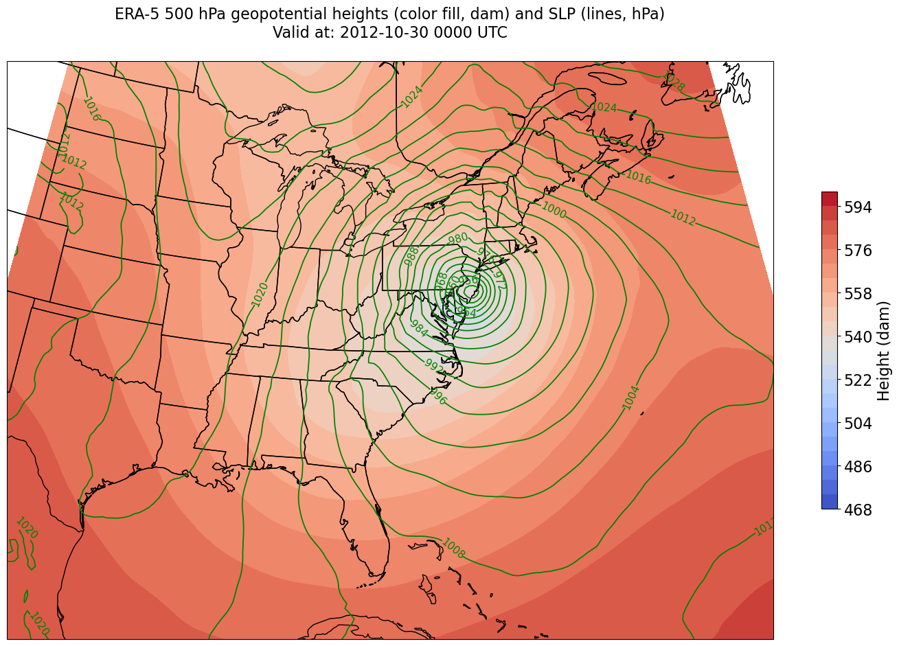
We’re missing the outer longitudes at higher latitudes. This is a consequence of reprojecting our data from PlateCarree to Lambert Conformal. We could do one of two things to resolve this:
Re-subset our original datset by extending the longitudinal ranges
Slightly constrain the map plotting region
Let’s use the latter method. The determination of how many degrees longitude to constrain is a process of trial and error; you want to avoid any blank areas in your map, but not restrict your map domain so much that you lose features at the edge of your map.
constrainLon = 3.3 # trial and error!

fig = plt.figure(figsize=(18,12))
ax = plt.subplot(1,1,1,projection=proj_map)
ax.set_extent ([lonW+constrainLon,lonE-constrainLon,latS,latN])
ax.add_feature(cfeature.COASTLINE.with_scale(res))
ax.add_feature(cfeature.STATES.with_scale(res))

CF = ax.contourf(lons,lats,HGHT, levels=HGHTcintervals,transform=proj_data,cmap=plt.get_cmap('coolwarm'))
cbar = plt.colorbar(CF,shrink=0.5)
cbar.ax.tick_params(labelsize=16)
cbar.ax.set_ylabel("Height (dam)",fontsize=16)

CL = ax.contour(lons,lats,SLP,SLPcintervals,transform=proj_data,linewidths=1.25,colors='green')
ax.clabel(CL, inline_spacing=0.2, fontsize=11, fmt='%.0f')
title = ax.set_title(title_line,fontsize=16)
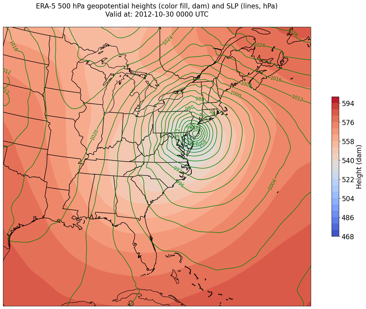
Summary
Via the OpenDAP protocol, Xarray can open remotely-served datasets, such as the ERA-5 from the RDA THREDDS server.
Subsetting our data request results in less data being transferred, as well as more consistent contour labels.
What’s Next?
We’ll continue to work with the ERA-5 repository, constructing time series and performing more complicated diagnostic calculations.