LambertConformal_Projection
()
int32
...
grid_mapping_name : lambert_conformal_conic latitude_of_projection_origin : 25.0 longitude_of_central_meridian : 265.0 standard_parallel : 25.0 earth_radius : 6371229.0 _CoordinateTransformType : Projection _CoordinateAxisTypes : GeoX GeoY [1 values with dtype=int32] time1_bounds
(time1, time1_bounds_1)
datetime64[ns]
...
long_name : bounds for time1 [36 values with dtype=datetime64[ns]] time2_bounds
(time2, time2_bounds_1)
datetime64[ns]
...
long_name : bounds for time2 [38 values with dtype=datetime64[ns]] pressure_difference_layer_bounds
(pressure_difference_layer, pressure_difference_layer_bounds_1)
float32
...
units : Pa long_name : bounds for pressure_difference_layer [2 values with dtype=float32] pressure_difference_layer1_bounds
(pressure_difference_layer1, pressure_difference_layer1_bounds_1)
float32
...
units : Pa long_name : bounds for pressure_difference_layer1 [2 values with dtype=float32] height_above_ground_layer_bounds
(height_above_ground_layer, height_above_ground_layer_bounds_1)
float32
...
units : m long_name : bounds for height_above_ground_layer [2 values with dtype=float32] height_above_ground_layer1_bounds
(height_above_ground_layer1, height_above_ground_layer1_bounds_1)
float32
...
units : m long_name : bounds for height_above_ground_layer1 [2 values with dtype=float32] height_above_ground_layer2_bounds
(height_above_ground_layer2, height_above_ground_layer2_bounds_1)
float32
...
units : m long_name : bounds for height_above_ground_layer2 [4 values with dtype=float32] pressure_difference_layer2_bounds
(pressure_difference_layer2, pressure_difference_layer2_bounds_1)
float32
...
units : Pa long_name : bounds for pressure_difference_layer2 [2 values with dtype=float32] height_above_ground_layer3_bounds
(height_above_ground_layer3, height_above_ground_layer3_bounds_1)
float32
...
units : m long_name : bounds for height_above_ground_layer3 [4 values with dtype=float32] isobaric_layer_bounds
(isobaric_layer, isobaric_layer_bounds_1)
float32
...
units : Pa long_name : bounds for isobaric_layer [2 values with dtype=float32] sigma_layer_bounds
(sigma_layer, sigma_layer_bounds_1)
float32
...
units : sigma long_name : bounds for sigma_layer [2 values with dtype=float32] pressure_difference_layer3_bounds
(pressure_difference_layer3, pressure_difference_layer3_bounds_1)
float32
...
units : Pa long_name : bounds for pressure_difference_layer3 [4 values with dtype=float32] Categorical_freezing_rain_surface
(time, y, x)
float32
...
long_name : Categorical freezing rain @ Ground or water surface units : (Code table 4.222) abbreviation : CFRZR grid_mapping : LambertConformal_Projection Grib_Variable_Id : VAR_0-1-34_L1 Grib2_Parameter : [ 0 1 34] Grib2_Parameter_Discipline : Meteorological products Grib2_Parameter_Category : Moisture Grib2_Parameter_Name : Categorical freezing rain Grib2_Level_Type : 1 Grib2_Level_Desc : Ground or water surface Grib2_Generating_Process_Type : Forecast Grib2_Statistical_Process_Type : UnknownStatType--1 [56119635 values with dtype=float32] Categorical_ice_pellets_surface
(time, y, x)
float32
...
long_name : Categorical ice pellets @ Ground or water surface units : (Code table 4.222) abbreviation : CICEP grid_mapping : LambertConformal_Projection Grib_Variable_Id : VAR_0-1-35_L1 Grib2_Parameter : [ 0 1 35] Grib2_Parameter_Discipline : Meteorological products Grib2_Parameter_Category : Moisture Grib2_Parameter_Name : Categorical ice pellets Grib2_Level_Type : 1 Grib2_Level_Desc : Ground or water surface Grib2_Generating_Process_Type : Forecast Grib2_Statistical_Process_Type : UnknownStatType--1 [56119635 values with dtype=float32] Categorical_rain_surface
(time, y, x)
float32
...
long_name : Categorical rain @ Ground or water surface units : (Code table 4.222) abbreviation : CRAIN grid_mapping : LambertConformal_Projection Grib_Variable_Id : VAR_0-1-33_L1 Grib2_Parameter : [ 0 1 33] Grib2_Parameter_Discipline : Meteorological products Grib2_Parameter_Category : Moisture Grib2_Parameter_Name : Categorical rain Grib2_Level_Type : 1 Grib2_Level_Desc : Ground or water surface Grib2_Generating_Process_Type : Forecast Grib2_Statistical_Process_Type : UnknownStatType--1 [56119635 values with dtype=float32] Categorical_snow_surface
(time, y, x)
float32
...
long_name : Categorical snow @ Ground or water surface units : (Code table 4.222) abbreviation : CSNOW grid_mapping : LambertConformal_Projection Grib_Variable_Id : VAR_0-1-36_L1 Grib2_Parameter : [ 0 1 36] Grib2_Parameter_Discipline : Meteorological products Grib2_Parameter_Category : Moisture Grib2_Parameter_Name : Categorical snow Grib2_Level_Type : 1 Grib2_Level_Desc : Ground or water surface Grib2_Generating_Process_Type : Forecast Grib2_Statistical_Process_Type : UnknownStatType--1 [56119635 values with dtype=float32] Convective_available_potential_energy_pressure_difference_layer
(time, pressure_difference_layer3, y, x)
float32
...
long_name : Convective available potential energy @ Level at specified pressure difference from ground to level layer units : J/kg abbreviation : CAPE grid_mapping : LambertConformal_Projection Grib_Variable_Id : VAR_0-7-6_L108_layer Grib2_Parameter : [0 7 6] Grib2_Parameter_Discipline : Meteorological products Grib2_Parameter_Category : Thermodynamic stability indices Grib2_Parameter_Name : Convective available potential energy Grib2_Level_Type : 108 Grib2_Level_Desc : Level at specified pressure difference from ground to level Grib2_Generating_Process_Type : Forecast Grib2_Statistical_Process_Type : UnknownStatType--1 [112239270 values with dtype=float32] Convective_available_potential_energy_surface
(time, y, x)
float32
...
long_name : Convective available potential energy @ Ground or water surface units : J/kg abbreviation : CAPE grid_mapping : LambertConformal_Projection Grib_Variable_Id : VAR_0-7-6_L1 Grib2_Parameter : [0 7 6] Grib2_Parameter_Discipline : Meteorological products Grib2_Parameter_Category : Thermodynamic stability indices Grib2_Parameter_Name : Convective available potential energy Grib2_Level_Type : 1 Grib2_Level_Desc : Ground or water surface Grib2_Generating_Process_Type : Forecast Grib2_Statistical_Process_Type : UnknownStatType--1 [56119635 values with dtype=float32] Convective_inhibition_pressure_difference_layer
(time, pressure_difference_layer3, y, x)
float32
...
long_name : Convective inhibition @ Level at specified pressure difference from ground to level layer units : J/kg abbreviation : CIN grid_mapping : LambertConformal_Projection Grib_Variable_Id : VAR_0-7-7_L108_layer Grib2_Parameter : [0 7 7] Grib2_Parameter_Discipline : Meteorological products Grib2_Parameter_Category : Thermodynamic stability indices Grib2_Parameter_Name : Convective inhibition Grib2_Level_Type : 108 Grib2_Level_Desc : Level at specified pressure difference from ground to level Grib2_Generating_Process_Type : Forecast Grib2_Statistical_Process_Type : UnknownStatType--1 [112239270 values with dtype=float32] Convective_inhibition_surface
(time, y, x)
float32
...
long_name : Convective inhibition @ Ground or water surface units : J/kg abbreviation : CIN grid_mapping : LambertConformal_Projection Grib_Variable_Id : VAR_0-7-7_L1 Grib2_Parameter : [0 7 7] Grib2_Parameter_Discipline : Meteorological products Grib2_Parameter_Category : Thermodynamic stability indices Grib2_Parameter_Name : Convective inhibition Grib2_Level_Type : 1 Grib2_Level_Desc : Ground or water surface Grib2_Generating_Process_Type : Forecast Grib2_Statistical_Process_Type : UnknownStatType--1 [56119635 values with dtype=float32] Dewpoint_temperature_isobaric
(time, isobaric1, y, x)
float32
...
long_name : Dewpoint temperature @ Isobaric surface units : K abbreviation : DPT grid_mapping : LambertConformal_Projection Grib_Variable_Id : VAR_0-0-6_L100 Grib2_Parameter : [0 0 6] Grib2_Parameter_Discipline : Meteorological products Grib2_Parameter_Category : Temperature Grib2_Parameter_Name : Dewpoint temperature Grib2_Level_Type : 100 Grib2_Level_Desc : Isobaric surface Grib2_Generating_Process_Type : Forecast Grib2_Statistical_Process_Type : UnknownStatType--1 [280598175 values with dtype=float32] Dewpoint_temperature_height_above_ground
(time, height_above_ground3, y, x)
float32
...
long_name : Dewpoint temperature @ Specified height level above ground units : K abbreviation : DPT grid_mapping : LambertConformal_Projection Grib_Variable_Id : VAR_0-0-6_L103 Grib2_Parameter : [0 0 6] Grib2_Parameter_Discipline : Meteorological products Grib2_Parameter_Category : Temperature Grib2_Parameter_Name : Dewpoint temperature Grib2_Level_Type : 103 Grib2_Level_Desc : Specified height level above ground Grib2_Generating_Process_Type : Forecast Grib2_Statistical_Process_Type : UnknownStatType--1 [56119635 values with dtype=float32] Echo_top_cloud_tops
(time, y, x)
float32
...
long_name : Echo top @ Level of cloud tops units : m abbreviation : RETOP grid_mapping : LambertConformal_Projection Grib_Variable_Id : VAR_0-16-3_L3 Grib2_Parameter : [ 0 16 3] Grib2_Parameter_Discipline : Meteorological products Grib2_Parameter_Category : Forecast Radar Imagery Grib2_Parameter_Name : Echo top Grib2_Level_Type : 3 Grib2_Level_Desc : Level of cloud tops Grib2_Generating_Process_Type : Forecast Grib2_Statistical_Process_Type : UnknownStatType--1 [56119635 values with dtype=float32] Geopotential_height_isobaric
(time, isobaric, y, x)
float32
...
long_name : Geopotential height @ Isobaric surface units : gpm abbreviation : HGT grid_mapping : LambertConformal_Projection Grib_Variable_Id : VAR_0-3-5_L100 Grib2_Parameter : [0 3 5] Grib2_Parameter_Discipline : Meteorological products Grib2_Parameter_Category : Mass Grib2_Parameter_Name : Geopotential height Grib2_Level_Type : 100 Grib2_Level_Desc : Isobaric surface Grib2_Generating_Process_Type : Forecast Grib2_Statistical_Process_Type : UnknownStatType--1 [224478540 values with dtype=float32] Geopotential_height_adiabatic_condensation_lifted
(time, y, x)
float32
...
long_name : Geopotential height @ Level of adiabatic condensation lifted from the surface units : gpm abbreviation : HGT grid_mapping : LambertConformal_Projection Grib_Variable_Id : VAR_0-3-5_L5 Grib2_Parameter : [0 3 5] Grib2_Parameter_Discipline : Meteorological products Grib2_Parameter_Category : Mass Grib2_Parameter_Name : Geopotential height Grib2_Level_Type : 5 Grib2_Level_Desc : Level of adiabatic condensation lifted from the surface Grib2_Generating_Process_Type : Forecast Grib2_Statistical_Process_Type : UnknownStatType--1 [56119635 values with dtype=float32] Geopotential_height_cloud_ceiling
(time, y, x)
float32
...
long_name : Geopotential height @ Cloud ceiling units : gpm abbreviation : HGT grid_mapping : LambertConformal_Projection Grib_Variable_Id : VAR_0-3-5_L215 Grib2_Parameter : [0 3 5] Grib2_Parameter_Discipline : Meteorological products Grib2_Parameter_Category : Mass Grib2_Parameter_Name : Geopotential height Grib2_Level_Type : 215 Grib2_Level_Desc : Cloud ceiling Grib2_Generating_Process_Type : Forecast Grib2_Statistical_Process_Type : UnknownStatType--1 [56119635 values with dtype=float32] Geopotential_height_surface
(time, y, x)
float32
...
long_name : Geopotential height @ Ground or water surface units : gpm abbreviation : HGT grid_mapping : LambertConformal_Projection Grib_Variable_Id : VAR_0-3-5_L1 Grib2_Parameter : [0 3 5] Grib2_Parameter_Discipline : Meteorological products Grib2_Parameter_Category : Mass Grib2_Parameter_Name : Geopotential height Grib2_Level_Type : 1 Grib2_Level_Desc : Ground or water surface Grib2_Generating_Process_Type : Forecast Grib2_Statistical_Process_Type : UnknownStatType--1 [56119635 values with dtype=float32] Geopotential_height_cloud_tops
(time, y, x)
float32
...
long_name : Geopotential height @ Level of cloud tops units : gpm abbreviation : HGT grid_mapping : LambertConformal_Projection Grib_Variable_Id : VAR_0-3-5_L3 Grib2_Parameter : [0 3 5] Grib2_Parameter_Discipline : Meteorological products Grib2_Parameter_Category : Mass Grib2_Parameter_Name : Geopotential height Grib2_Level_Type : 3 Grib2_Level_Desc : Level of cloud tops Grib2_Generating_Process_Type : Forecast Grib2_Statistical_Process_Type : UnknownStatType--1 [56119635 values with dtype=float32] High_cloud_cover_high_cloud
(time, y, x)
float32
...
long_name : High cloud cover @ High cloud layer units : % abbreviation : HCDC grid_mapping : LambertConformal_Projection Grib_Variable_Id : VAR_0-6-5_L234 Grib2_Parameter : [0 6 5] Grib2_Parameter_Discipline : Meteorological products Grib2_Parameter_Category : Cloud Grib2_Parameter_Name : High cloud cover Grib2_Level_Type : 234 Grib2_Level_Desc : High cloud layer Grib2_Generating_Process_Type : Forecast Grib2_Statistical_Process_Type : UnknownStatType--1 [56119635 values with dtype=float32] Low_cloud_cover_low_cloud
(time, y, x)
float32
...
long_name : Low cloud cover @ Low cloud layer units : % abbreviation : LCDC grid_mapping : LambertConformal_Projection Grib_Variable_Id : VAR_0-6-3_L214 Grib2_Parameter : [0 6 3] Grib2_Parameter_Discipline : Meteorological products Grib2_Parameter_Category : Cloud Grib2_Parameter_Name : Low cloud cover Grib2_Level_Type : 214 Grib2_Level_Desc : Low cloud layer Grib2_Generating_Process_Type : Forecast Grib2_Statistical_Process_Type : UnknownStatType--1 [56119635 values with dtype=float32] Medium_cloud_cover_middle_cloud
(time, y, x)
float32
...
long_name : Medium cloud cover @ Middle cloud layer units : % abbreviation : MCDC grid_mapping : LambertConformal_Projection Grib_Variable_Id : VAR_0-6-4_L224 Grib2_Parameter : [0 6 4] Grib2_Parameter_Discipline : Meteorological products Grib2_Parameter_Category : Cloud Grib2_Parameter_Name : Medium cloud cover Grib2_Level_Type : 224 Grib2_Level_Desc : Middle cloud layer Grib2_Generating_Process_Type : Forecast Grib2_Statistical_Process_Type : UnknownStatType--1 [56119635 values with dtype=float32] Per_cent_frozen_precipitation_surface
(time, y, x)
float32
...
long_name : Per cent frozen precipitation @ Ground or water surface units : % abbreviation : CPOFP grid_mapping : LambertConformal_Projection Grib_Variable_Id : VAR_0-1-39_L1 Grib2_Parameter : [ 0 1 39] Grib2_Parameter_Discipline : Meteorological products Grib2_Parameter_Category : Moisture Grib2_Parameter_Name : Per cent frozen precipitation Grib2_Level_Type : 1 Grib2_Level_Desc : Ground or water surface Grib2_Generating_Process_Type : Forecast Grib2_Statistical_Process_Type : UnknownStatType--1 [56119635 values with dtype=float32] Planetary_boundary_layer_height_surface
(time, y, x)
float32
...
long_name : Planetary boundary layer height @ Ground or water surface units : m abbreviation : HPBL grid_mapping : LambertConformal_Projection Grib_Variable_Id : VAR_0-3-18_L1 Grib2_Parameter : [ 0 3 18] Grib2_Parameter_Discipline : Meteorological products Grib2_Parameter_Category : Mass Grib2_Parameter_Name : Planetary boundary layer height Grib2_Level_Type : 1 Grib2_Level_Desc : Ground or water surface Grib2_Generating_Process_Type : Forecast Grib2_Statistical_Process_Type : UnknownStatType--1 [56119635 values with dtype=float32] Precipitable_water_entire_atmosphere_single_layer
(time, y, x)
float32
...
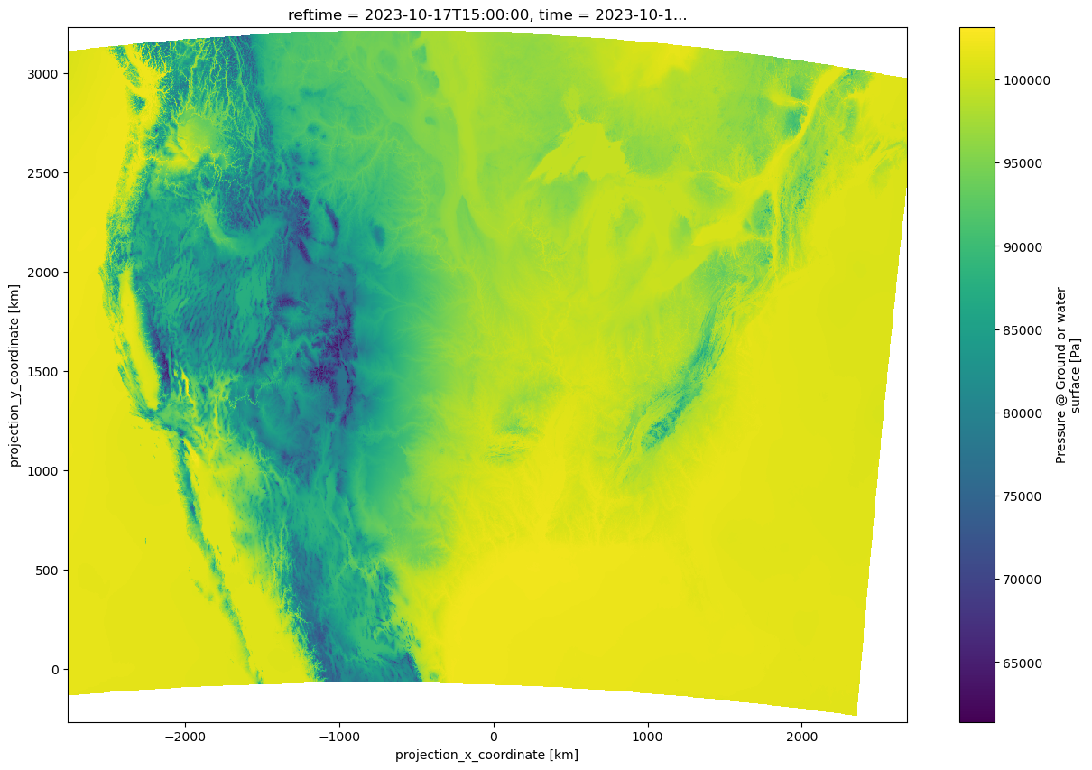
long_name : Precipitable water @ Entire atmosphere layer units : kg.m-2 abbreviation : PWAT grid_mapping : LambertConformal_Projection Grib_Variable_Id : VAR_0-1-3_L200 Grib2_Parameter : [0 1 3] Grib2_Parameter_Discipline : Meteorological products Grib2_Parameter_Category : Moisture Grib2_Parameter_Name : Precipitable water Grib2_Level_Type : 200 Grib2_Level_Desc : Entire atmosphere layer Grib2_Generating_Process_Type : Forecast Grib2_Statistical_Process_Type : UnknownStatType--1 [56119635 values with dtype=float32] Pressure_surface
(time, y, x)
float32
...
long_name : Pressure @ Ground or water surface units : Pa abbreviation : PRES grid_mapping : LambertConformal_Projection Grib_Variable_Id : VAR_0-3-0_L1 Grib2_Parameter : [0 3 0] Grib2_Parameter_Discipline : Meteorological products Grib2_Parameter_Category : Mass Grib2_Parameter_Name : Pressure Grib2_Level_Type : 1 Grib2_Level_Desc : Ground or water surface Grib2_Generating_Process_Type : Forecast Grib2_Statistical_Process_Type : UnknownStatType--1 [56119635 values with dtype=float32] Pressure_reduced_to_MSL_msl
(time, y, x)
float32
...
long_name : Pressure reduced to MSL @ Mean sea level units : Pa abbreviation : PRMSL grid_mapping : LambertConformal_Projection Grib_Variable_Id : VAR_0-3-1_L101 Grib2_Parameter : [0 3 1] Grib2_Parameter_Discipline : Meteorological products Grib2_Parameter_Category : Mass Grib2_Parameter_Name : Pressure reduced to MSL Grib2_Level_Type : 101 Grib2_Level_Desc : Mean sea level Grib2_Generating_Process_Type : Forecast Grib2_Statistical_Process_Type : UnknownStatType--1 [56119635 values with dtype=float32] Snow_depth_surface
(time, y, x)
float32
...
long_name : Snow depth @ Ground or water surface units : m abbreviation : SNOD grid_mapping : LambertConformal_Projection Grib_Variable_Id : VAR_0-1-11_L1 Grib2_Parameter : [ 0 1 11] Grib2_Parameter_Discipline : Meteorological products Grib2_Parameter_Category : Moisture Grib2_Parameter_Name : Snow depth Grib2_Level_Type : 1 Grib2_Level_Desc : Ground or water surface Grib2_Generating_Process_Type : Forecast Grib2_Statistical_Process_Type : UnknownStatType--1 [56119635 values with dtype=float32] Storm_relative_helicity_height_above_ground_layer
(time, height_above_ground_layer2, y, x)
float32
...
long_name : Storm relative helicity @ Specified height level above ground layer units : J/kg abbreviation : HLCY grid_mapping : LambertConformal_Projection Grib_Variable_Id : VAR_0-7-8_L103_layer Grib2_Parameter : [0 7 8] Grib2_Parameter_Discipline : Meteorological products Grib2_Parameter_Category : Thermodynamic stability indices Grib2_Parameter_Name : Storm relative helicity Grib2_Level_Type : 103 Grib2_Level_Desc : Specified height level above ground Grib2_Generating_Process_Type : Forecast Grib2_Statistical_Process_Type : UnknownStatType--1 [112239270 values with dtype=float32] Surface_lifted_index_isobaric_layer
(time, isobaric_layer, y, x)
float32
...
long_name : Surface lifted index @ Isobaric surface layer units : K abbreviation : LFT X grid_mapping : LambertConformal_Projection Grib_Variable_Id : VAR_0-7-10_L100_layer Grib2_Parameter : [ 0 7 10] Grib2_Parameter_Discipline : Meteorological products Grib2_Parameter_Category : Thermodynamic stability indices Grib2_Parameter_Name : Surface lifted index Grib2_Level_Type : 100 Grib2_Level_Desc : Isobaric surface Grib2_Generating_Process_Type : Forecast Grib2_Statistical_Process_Type : UnknownStatType--1 [56119635 values with dtype=float32] Temperature_isobaric
(time, isobaric1, y, x)
float32
...
long_name : Temperature @ Isobaric surface units : K abbreviation : TMP grid_mapping : LambertConformal_Projection Grib_Variable_Id : VAR_0-0-0_L100 Grib2_Parameter : [0 0 0] Grib2_Parameter_Discipline : Meteorological products Grib2_Parameter_Category : Temperature Grib2_Parameter_Name : Temperature Grib2_Level_Type : 100 Grib2_Level_Desc : Isobaric surface Grib2_Generating_Process_Type : Forecast Grib2_Statistical_Process_Type : UnknownStatType--1 [280598175 values with dtype=float32] Temperature_height_above_ground
(time, height_above_ground3, y, x)
float32
...
long_name : Temperature @ Specified height level above ground units : K abbreviation : TMP grid_mapping : LambertConformal_Projection Grib_Variable_Id : VAR_0-0-0_L103 Grib2_Parameter : [0 0 0] Grib2_Parameter_Discipline : Meteorological products Grib2_Parameter_Category : Temperature Grib2_Parameter_Name : Temperature Grib2_Level_Type : 103 Grib2_Level_Desc : Specified height level above ground Grib2_Generating_Process_Type : Forecast Grib2_Statistical_Process_Type : UnknownStatType--1 [56119635 values with dtype=float32] Total_cloud_cover_entire_atmosphere
(time, y, x)
float32
...
long_name : Total cloud cover @ Entire atmosphere units : % abbreviation : TCDC grid_mapping : LambertConformal_Projection Grib_Variable_Id : VAR_0-6-1_L10 Grib2_Parameter : [0 6 1] Grib2_Parameter_Discipline : Meteorological products Grib2_Parameter_Category : Cloud Grib2_Parameter_Name : Total cloud cover Grib2_Level_Type : 10 Grib2_Level_Desc : Entire atmosphere Grib2_Generating_Process_Type : Forecast Grib2_Statistical_Process_Type : UnknownStatType--1 [56119635 values with dtype=float32] Total_column_integrated_graupel_entire_atmosphere_single_layer_Mixed_intervals_Maximum
(time2, y, x)
float32
...
long_name : Total column integrated graupel (Mixed_intervals Maximum) @ Entire atmosphere layer units : kg.m-2 abbreviation : TCOLG grid_mapping : LambertConformal_Projection Grib_Statistical_Interval_Type : Maximum Grib_Variable_Id : VAR_0-1-74_L200_Imixed_S2 Grib2_Parameter : [ 0 1 74] Grib2_Parameter_Discipline : Meteorological products Grib2_Parameter_Category : Moisture Grib2_Parameter_Name : Total column integrated graupel Grib2_Level_Type : 200 Grib2_Level_Desc : Entire atmosphere layer Grib2_Generating_Process_Type : Forecast Grib2_Statistical_Process_Type : Maximum [56119635 values with dtype=float32] Total_precipitation_surface_1_Hour_Accumulation
(time1, y, x)
float32
...
long_name : Total precipitation (1_Hour Accumulation) @ Ground or water surface units : kg.m-2 abbreviation : APCP grid_mapping : LambertConformal_Projection Grib_Statistical_Interval_Type : Accumulation Grib_Variable_Id : VAR_0-1-8_L1_I1_Hour_S1 Grib2_Parameter : [0 1 8] Grib2_Parameter_Discipline : Meteorological products Grib2_Parameter_Category : Moisture Grib2_Parameter_Name : Total precipitation Grib2_Level_Type : 1 Grib2_Level_Desc : Ground or water surface Grib2_Generating_Process_Type : Forecast Grib2_Statistical_Process_Type : Accumulation [53165970 values with dtype=float32] Reflectivity_height_above_ground
(time, height_above_ground1, y, x)
float32
...
long_name : Reflectivity @ Specified height level above ground units : dB abbreviation : REFD grid_mapping : LambertConformal_Projection Grib_Variable_Id : VAR_0-16-195_L103 Grib2_Parameter : [ 0 16 195] Grib2_Parameter_Discipline : Meteorological products Grib2_Parameter_Category : Forecast Radar Imagery Grib2_Parameter_Name : Reflectivity Grib2_Level_Type : 103 Grib2_Level_Desc : Specified height level above ground Grib2_Generating_Process_Type : Forecast Grib2_Statistical_Process_Type : UnknownStatType--1 [56119635 values with dtype=float32] Composite_reflectivity_entire_atmosphere
(time, y, x)
float32
...
long_name : Composite reflectivity @ Entire atmosphere units : dB abbreviation : REFC grid_mapping : LambertConformal_Projection Grib_Variable_Id : VAR_0-16-196_L10 Grib2_Parameter : [ 0 16 196] Grib2_Parameter_Discipline : Meteorological products Grib2_Parameter_Category : Forecast Radar Imagery Grib2_Parameter_Name : Composite reflectivity Grib2_Level_Type : 10 Grib2_Level_Desc : Entire atmosphere Grib2_Generating_Process_Type : Forecast Grib2_Statistical_Process_Type : UnknownStatType--1 [56119635 values with dtype=float32] Hourly_Maximum_of_Simulated_Reflectivity_at_1_km_AGL_height_above_ground_Mixed_intervals_Maximum
(time2, height_above_ground1, y, x)
float32
...
long_name : Hourly Maximum of Simulated Reflectivity at 1 km AGL (Mixed_intervals Maximum) @ Specified height level above ground units : dB abbreviation : MAXREF grid_mapping : LambertConformal_Projection Grib_Statistical_Interval_Type : Maximum Grib_Variable_Id : VAR_0-16-198_L103_Imixed_S2 Grib2_Parameter : [ 0 16 198] Grib2_Parameter_Discipline : Meteorological products Grib2_Parameter_Category : Forecast Radar Imagery Grib2_Parameter_Name : Hourly Maximum of Simulated Reflectivity at 1 km AGL Grib2_Level_Type : 103 Grib2_Level_Desc : Specified height level above ground Grib2_Generating_Process_Type : Forecast Grib2_Statistical_Process_Type : Maximum [56119635 values with dtype=float32] Lightning_entire_atmosphere
(time, y, x)
float32
...
long_name : Lightning @ Entire atmosphere units : non-dim abbreviation : LTNG grid_mapping : LambertConformal_Projection Grib_Variable_Id : VAR_0-17-192_L10 Grib2_Parameter : [ 0 17 192] Grib2_Parameter_Discipline : Meteorological products Grib2_Parameter_Category : Electrodynamics Grib2_Parameter_Name : Lightning Grib2_Level_Type : 10 Grib2_Level_Desc : Entire atmosphere Grib2_Generating_Process_Type : Forecast Grib2_Statistical_Process_Type : UnknownStatType--1 [56119635 values with dtype=float32] Hourly_Maximum_of_Upward_Vertical_Velocity_in_the_lowest_400hPa_pressure_difference_layer_Mixed_intervals_Maximum
(time2, pressure_difference_layer2, y, x)
float32
...
long_name : Hourly Maximum of Upward Vertical Velocity in the lowest 400hPa (Mixed_intervals Maximum) @ Level at specified pressure difference from ground to level layer units : m.s-1 abbreviation : MAXUVV grid_mapping : LambertConformal_Projection Grib_Statistical_Interval_Type : Maximum Grib_Variable_Id : VAR_0-2-220_L108_layer_Imixed_S2 Grib2_Parameter : [ 0 2 220] Grib2_Parameter_Discipline : Meteorological products Grib2_Parameter_Category : Momentum Grib2_Parameter_Name : Hourly Maximum of Upward Vertical Velocity in the lowest 400hPa Grib2_Level_Type : 108 Grib2_Level_Desc : Level at specified pressure difference from ground to level Grib2_Generating_Process_Type : Forecast Grib2_Statistical_Process_Type : Maximum [56119635 values with dtype=float32] Hourly_Maximum_of_Downward_Vertical_Velocity_in_the_lowest_400hPa_pressure_difference_layer_Mixed_intervals_Maximum
(time2, pressure_difference_layer2, y, x)
float32
...
long_name : Hourly Maximum of Downward Vertical Velocity in the lowest 400hPa (Mixed_intervals Maximum) @ Level at specified pressure difference from ground to level layer units : m.s-1 abbreviation : MAXDVV grid_mapping : LambertConformal_Projection Grib_Statistical_Interval_Type : Maximum Grib_Variable_Id : VAR_0-2-221_L108_layer_Imixed_S2 Grib2_Parameter : [ 0 2 221] Grib2_Parameter_Discipline : Meteorological products Grib2_Parameter_Category : Momentum Grib2_Parameter_Name : Hourly Maximum of Downward Vertical Velocity in the lowest 400hPa Grib2_Level_Type : 108 Grib2_Level_Desc : Level at specified pressure difference from ground to level Grib2_Generating_Process_Type : Forecast Grib2_Statistical_Process_Type : Maximum [56119635 values with dtype=float32] Pressure_of_level_from_which_parcel_was_lifted_pressure_difference_layer
(time, pressure_difference_layer, y, x)
float32
...
long_name : Pressure of level from which parcel was lifted @ Level at specified pressure difference from ground to level layer units : Pa abbreviation : PLPL grid_mapping : LambertConformal_Projection Grib_Variable_Id : VAR_0-3-200_L108_layer Grib2_Parameter : [ 0 3 200] Grib2_Parameter_Discipline : Meteorological products Grib2_Parameter_Category : Mass Grib2_Parameter_Name : Pressure of level from which parcel was lifted Grib2_Level_Type : 108 Grib2_Level_Desc : Level at specified pressure difference from ground to level Grib2_Generating_Process_Type : Forecast Grib2_Statistical_Process_Type : UnknownStatType--1 [56119635 values with dtype=float32] Best_4_layer_Lifted_Index_pressure_difference_layer
(time, pressure_difference_layer1, y, x)
float32
...
long_name : Best (4 layer) Lifted Index @ Level at specified pressure difference from ground to level layer units : K abbreviation : 4LFTX grid_mapping : LambertConformal_Projection Grib_Variable_Id : VAR_0-7-193_L108_layer Grib2_Parameter : [ 0 7 193] Grib2_Parameter_Discipline : Meteorological products Grib2_Parameter_Category : Thermodynamic stability indices Grib2_Parameter_Name : Best (4 layer) Lifted Index Grib2_Level_Type : 108 Grib2_Level_Desc : Level at specified pressure difference from ground to level Grib2_Generating_Process_Type : Forecast Grib2_Statistical_Process_Type : UnknownStatType--1 [56119635 values with dtype=float32] Hourly_Maximum_of_Updraft_Helicity_over_Layer_2km_to_5_km_AGL_height_above_ground_layer_Mixed_intervals_Maximum
(time2, height_above_ground_layer, y, x)
float32
...
long_name : Hourly Maximum of Updraft Helicity over Layer 2km to 5 km AGL (Mixed_intervals Maximum) @ Specified height level above ground layer units : m2.s-2 abbreviation : MXUPHL grid_mapping : LambertConformal_Projection Grib_Statistical_Interval_Type : Maximum Grib_Variable_Id : VAR_0-7-199_L103_layer_Imixed_S2 Grib2_Parameter : [ 0 7 199] Grib2_Parameter_Discipline : Meteorological products Grib2_Parameter_Category : Thermodynamic stability indices Grib2_Parameter_Name : Hourly Maximum of Updraft Helicity over Layer 2km to 5 km AGL Grib2_Level_Type : 103 Grib2_Level_Desc : Specified height level above ground Grib2_Generating_Process_Type : Forecast Grib2_Statistical_Process_Type : Maximum [56119635 values with dtype=float32] Vertical_u-component_shear_height_above_ground_layer
(time, height_above_ground_layer3, y, x)
float32
...
long_name : Vertical u-component shear @ Specified height level above ground layer units : 1/s abbreviation : VUCSH grid_mapping : LambertConformal_Projection Grib_Variable_Id : VAR_0-2-15_L103_layer Grib2_Parameter : [ 0 2 15] Grib2_Parameter_Discipline : Meteorological products Grib2_Parameter_Category : Momentum Grib2_Parameter_Name : Vertical u-component shear Grib2_Level_Type : 103 Grib2_Level_Desc : Specified height level above ground Grib2_Generating_Process_Type : Forecast Grib2_Statistical_Process_Type : UnknownStatType--1 [112239270 values with dtype=float32] Vertical_v-component_shear_height_above_ground_layer
(time, height_above_ground_layer3, y, x)
float32
...
long_name : Vertical v-component shear @ Specified height level above ground layer units : 1/s abbreviation : VVCSH grid_mapping : LambertConformal_Projection Grib_Variable_Id : VAR_0-2-16_L103_layer Grib2_Parameter : [ 0 2 16] Grib2_Parameter_Discipline : Meteorological products Grib2_Parameter_Category : Momentum Grib2_Parameter_Name : Vertical v-component shear Grib2_Level_Type : 103 Grib2_Level_Desc : Specified height level above ground Grib2_Generating_Process_Type : Forecast Grib2_Statistical_Process_Type : UnknownStatType--1 [112239270 values with dtype=float32] Vertical_velocity_geometric_sigma_layer_Mixed_intervals_Average
(time2, sigma_layer, y, x)
float32
...
long_name : Vertical velocity (geometric) (Mixed_intervals Average) @ Sigma level layer units : m/s abbreviation : DZDT grid_mapping : LambertConformal_Projection Grib_Statistical_Interval_Type : Average Grib_Variable_Id : VAR_0-2-9_L104_layer_Imixed_S0 Grib2_Parameter : [0 2 9] Grib2_Parameter_Discipline : Meteorological products Grib2_Parameter_Category : Momentum Grib2_Parameter_Name : Vertical velocity (geometric) Grib2_Level_Type : 104 Grib2_Level_Desc : Sigma level Grib2_Generating_Process_Type : Forecast Grib2_Statistical_Process_Type : Average [56119635 values with dtype=float32] Vertically_integrated_liquid_water_VIL_entire_atmosphere
(time, y, x)
float32
...
long_name : Vertically integrated liquid water (VIL) @ Entire atmosphere units : kg.m-2 abbreviation : VIL grid_mapping : LambertConformal_Projection Grib_Variable_Id : VAR_0-15-3_L10 Grib2_Parameter : [ 0 15 3] Grib2_Parameter_Discipline : Meteorological products Grib2_Parameter_Category : Radar Grib2_Parameter_Name : Vertically integrated liquid water (VIL) Grib2_Level_Type : 10 Grib2_Level_Desc : Entire atmosphere Grib2_Generating_Process_Type : Forecast Grib2_Statistical_Process_Type : UnknownStatType--1 [56119635 values with dtype=float32] Visibility_surface
(time, y, x)
float32
...
long_name : Visibility @ Ground or water surface units : m abbreviation : VIS grid_mapping : LambertConformal_Projection Grib_Variable_Id : VAR_0-19-0_L1 Grib2_Parameter : [ 0 19 0] Grib2_Parameter_Discipline : Meteorological products Grib2_Parameter_Category : Physical atmospheric Properties Grib2_Parameter_Name : Visibility Grib2_Level_Type : 1 Grib2_Level_Desc : Ground or water surface Grib2_Generating_Process_Type : Forecast Grib2_Statistical_Process_Type : UnknownStatType--1 [56119635 values with dtype=float32] Water_equivalent_of_accumulated_snow_depth_surface_1_Hour_Accumulation
(time1, y, x)
float32
...
long_name : Water equivalent of accumulated snow depth (1_Hour Accumulation) @ Ground or water surface units : kg.m-2 abbreviation : WEASD grid_mapping : LambertConformal_Projection Grib_Statistical_Interval_Type : Accumulation Grib_Variable_Id : VAR_0-1-13_L1_I1_Hour_S1 Grib2_Parameter : [ 0 1 13] Grib2_Parameter_Discipline : Meteorological products Grib2_Parameter_Category : Moisture Grib2_Parameter_Name : Water equivalent of accumulated snow depth Grib2_Level_Type : 1 Grib2_Level_Desc : Ground or water surface Grib2_Generating_Process_Type : Forecast Grib2_Statistical_Process_Type : Accumulation [53165970 values with dtype=float32] Wind_speed_height_above_ground_Mixed_intervals_Maximum
(time2, height_above_ground, y, x)
float32
...
long_name : Wind speed (Mixed_intervals Maximum) @ Specified height level above ground units : m/s abbreviation : WIND grid_mapping : LambertConformal_Projection Grib_Statistical_Interval_Type : Maximum Grib_Variable_Id : VAR_0-2-1_L103_Imixed_S2 Grib2_Parameter : [0 2 1] Grib2_Parameter_Discipline : Meteorological products Grib2_Parameter_Category : Momentum Grib2_Parameter_Name : Wind speed Grib2_Level_Type : 103 Grib2_Level_Desc : Specified height level above ground Grib2_Generating_Process_Type : Forecast Grib2_Statistical_Process_Type : Maximum [56119635 values with dtype=float32] Wind_speed_gust_surface
(time, y, x)
float32
...
long_name : Wind speed (gust) @ Ground or water surface units : m/s abbreviation : GUST grid_mapping : LambertConformal_Projection Grib_Variable_Id : VAR_0-2-22_L1 Grib2_Parameter : [ 0 2 22] Grib2_Parameter_Discipline : Meteorological products Grib2_Parameter_Category : Momentum Grib2_Parameter_Name : Wind speed (gust) Grib2_Level_Type : 1 Grib2_Level_Desc : Ground or water surface Grib2_Generating_Process_Type : Forecast Grib2_Statistical_Process_Type : UnknownStatType--1 [56119635 values with dtype=float32] u-component_of_wind_isobaric
(time, isobaric1, y, x)
float32
...
long_name : u-component of wind @ Isobaric surface units : m/s abbreviation : UGRD grid_mapping : LambertConformal_Projection Grib_Variable_Id : VAR_0-2-2_L100 Grib2_Parameter : [0 2 2] Grib2_Parameter_Discipline : Meteorological products Grib2_Parameter_Category : Momentum Grib2_Parameter_Name : u-component of wind Grib2_Level_Type : 100 Grib2_Level_Desc : Isobaric surface Grib2_Generating_Process_Type : Forecast Grib2_Statistical_Process_Type : UnknownStatType--1 [280598175 values with dtype=float32] u-component_of_wind_height_above_ground
(time, height_above_ground2, y, x)
float32
...
long_name : u-component of wind @ Specified height level above ground units : m/s abbreviation : UGRD grid_mapping : LambertConformal_Projection Grib_Variable_Id : VAR_0-2-2_L103 Grib2_Parameter : [0 2 2] Grib2_Parameter_Discipline : Meteorological products Grib2_Parameter_Category : Momentum Grib2_Parameter_Name : u-component of wind Grib2_Level_Type : 103 Grib2_Level_Desc : Specified height level above ground Grib2_Generating_Process_Type : Forecast Grib2_Statistical_Process_Type : UnknownStatType--1 [112239270 values with dtype=float32] u-component_storm_motion_height_above_ground_layer
(time, height_above_ground_layer1, y, x)
float32
...
long_name : u-component storm motion @ Specified height level above ground layer units : m/s abbreviation : USTM grid_mapping : LambertConformal_Projection Grib_Variable_Id : VAR_0-2-27_L103_layer Grib2_Parameter : [ 0 2 27] Grib2_Parameter_Discipline : Meteorological products Grib2_Parameter_Category : Momentum Grib2_Parameter_Name : u-component storm motion Grib2_Level_Type : 103 Grib2_Level_Desc : Specified height level above ground Grib2_Generating_Process_Type : Forecast Grib2_Statistical_Process_Type : UnknownStatType--1 [56119635 values with dtype=float32] v-component_of_wind_isobaric
(time, isobaric1, y, x)
float32
...
long_name : v-component of wind @ Isobaric surface units : m/s abbreviation : VGRD grid_mapping : LambertConformal_Projection Grib_Variable_Id : VAR_0-2-3_L100 Grib2_Parameter : [0 2 3] Grib2_Parameter_Discipline : Meteorological products Grib2_Parameter_Category : Momentum Grib2_Parameter_Name : v-component of wind Grib2_Level_Type : 100 Grib2_Level_Desc : Isobaric surface Grib2_Generating_Process_Type : Forecast Grib2_Statistical_Process_Type : UnknownStatType--1 [280598175 values with dtype=float32] v-component_of_wind_height_above_ground
(time, height_above_ground2, y, x)
float32
...
long_name : v-component of wind @ Specified height level above ground units : m/s abbreviation : VGRD grid_mapping : LambertConformal_Projection Grib_Variable_Id : VAR_0-2-3_L103 Grib2_Parameter : [0 2 3] Grib2_Parameter_Discipline : Meteorological products Grib2_Parameter_Category : Momentum Grib2_Parameter_Name : v-component of wind Grib2_Level_Type : 103 Grib2_Level_Desc : Specified height level above ground Grib2_Generating_Process_Type : Forecast Grib2_Statistical_Process_Type : UnknownStatType--1 [112239270 values with dtype=float32] v-component_storm_motion_height_above_ground_layer
(time, height_above_ground_layer1, y, x)
float32
...
long_name : v-component storm motion @ Specified height level above ground layer units : m/s abbreviation : VSTM grid_mapping : LambertConformal_Projection Grib_Variable_Id : VAR_0-2-28_L103_layer Grib2_Parameter : [ 0 2 28] Grib2_Parameter_Discipline : Meteorological products Grib2_Parameter_Category : Momentum Grib2_Parameter_Name : v-component storm motion Grib2_Level_Type : 103 Grib2_Level_Desc : Specified height level above ground Grib2_Generating_Process_Type : Forecast Grib2_Statistical_Process_Type : UnknownStatType--1 [56119635 values with dtype=float32]