Xarray 5: Time Series
Contents
Xarray 5: Time Series
Overview
Work with an ERA-5
Datasethosted on NCAR’s Research Data ArchiveSubset the Dataset along its dimensions
Perform diagnostic calculations and unit conversions
Perform Split-Apply-Combine
Create and refine a time series plot of minimum SLP and maximum windspeed over the subsetted region
Imports
import xarray as xr
import pandas as pd
import numpy as np
from datetime import datetime as dt
from metpy.units import units
import metpy.calc as mpcalc
import cartopy.crs as ccrs
import cartopy.feature as cfeature
import matplotlib.pyplot as plt
from matplotlib.dates import DateFormatter, AutoDateLocator,HourLocator,DayLocator,MonthLocator
from matplotlib.ticker import (MultipleLocator, AutoMinorLocator)
import requests
Work with an ERA-5 Dataset hosted on NCAR’s Remote Data Archive
Create OpenDAP URLs pointing to the variables as they are stored in RDA’s THREDDS server
ds_urlu = 'https://thredds.rda.ucar.edu/thredds/dodsC/files/g/ds633.0/e5.oper.an.sfc/201210/e5.oper.an.sfc.128_165_10u.ll025sc.2012100100_2012103123.nc'
ds_urlv = 'https://thredds.rda.ucar.edu/thredds/dodsC/files/g/ds633.0/e5.oper.an.sfc/201210/e5.oper.an.sfc.128_166_10v.ll025sc.2012100100_2012103123.nc'
ds_urlp = 'https://thredds.rda.ucar.edu/thredds/dodsC/files/g/ds633.0/e5.oper.an.sfc/201210/e5.oper.an.sfc.128_151_msl.ll025sc.2012100100_2012103123.nc'
Now open the three files as separate Datasets
dsSLP = xr.open_dataset(ds_urlp)
dsU10 = xr.open_dataset(ds_urlu)
dsV10 = xr.open_dataset(ds_urlv)
Examine one of the Datasets.
dsU10
<xarray.Dataset>
Dimensions:    (latitude: 721, longitude: 1440, time: 744)
Coordinates:
  * latitude   (latitude) float64 90.0 89.75 89.5 89.25 ... -89.5 -89.75 -90.0
  * longitude  (longitude) float64 0.0 0.25 0.5 0.75 ... 359.0 359.2 359.5 359.8
  * time       (time) datetime64[ns] 2012-10-01 ... 2012-10-31T23:00:00
Data variables:
    utc_date   (time) int32 ...
    VAR_10U    (time, latitude, longitude) float32 ...
Attributes:
    _NCProperties:                   version=1|netcdflibversion=4.6.1|hdf5lib...
    DATA_SOURCE:                     ECMWF: https://cds.climate.copernicus.eu...
    NETCDF_CONVERSION:               CISL RDA: Conversion from ECMWF GRIB1 da...
    NETCDF_VERSION:                  4.6.1
    CONVERSION_PLATFORM:             Linux casper21 3.10.0-693.21.1.el7.x86_6...
    CONVERSION_DATE:                 Mon Aug 26 16:10:34 MDT 2019
    Conventions:                     CF-1.6
    NETCDF_COMPRESSION:              NCO: Precision-preserving compression to...
    history:                         Mon Aug 26 16:11:11 2019: ncks -4 --ppc ...
    NCO:                             netCDF Operators version 4.7.4 (http://n...
DODS_EXTRA.Unlimited_Dimension: timeCreate DataArray objects for each of the three variables in the Datasets.
slp = dsSLP['MSL']
u10 = dsU10['VAR_10U']
v10 = dsV10['VAR_10V']
Subset the Dataset along its dimensions.
As we did before, we will perform temporal and areal subsetting.
Take advantage of Pandas’ date/time methods. In this case, we will use Pandas date_range.
Let’s define a function whose output we will use to label our plotted time series.
timeRange = pd.date_range(start="2012-10-27 00:00",end="2012-10-31 00:00",freq='1H')
timeRange
DatetimeIndex(['2012-10-27 00:00:00', '2012-10-27 01:00:00',
               '2012-10-27 02:00:00', '2012-10-27 03:00:00',
               '2012-10-27 04:00:00', '2012-10-27 05:00:00',
               '2012-10-27 06:00:00', '2012-10-27 07:00:00',
               '2012-10-27 08:00:00', '2012-10-27 09:00:00',
               '2012-10-27 10:00:00', '2012-10-27 11:00:00',
               '2012-10-27 12:00:00', '2012-10-27 13:00:00',
               '2012-10-27 14:00:00', '2012-10-27 15:00:00',
               '2012-10-27 16:00:00', '2012-10-27 17:00:00',
               '2012-10-27 18:00:00', '2012-10-27 19:00:00',
               '2012-10-27 20:00:00', '2012-10-27 21:00:00',
               '2012-10-27 22:00:00', '2012-10-27 23:00:00',
               '2012-10-28 00:00:00', '2012-10-28 01:00:00',
               '2012-10-28 02:00:00', '2012-10-28 03:00:00',
               '2012-10-28 04:00:00', '2012-10-28 05:00:00',
               '2012-10-28 06:00:00', '2012-10-28 07:00:00',
               '2012-10-28 08:00:00', '2012-10-28 09:00:00',
               '2012-10-28 10:00:00', '2012-10-28 11:00:00',
               '2012-10-28 12:00:00', '2012-10-28 13:00:00',
               '2012-10-28 14:00:00', '2012-10-28 15:00:00',
               '2012-10-28 16:00:00', '2012-10-28 17:00:00',
               '2012-10-28 18:00:00', '2012-10-28 19:00:00',
               '2012-10-28 20:00:00', '2012-10-28 21:00:00',
               '2012-10-28 22:00:00', '2012-10-28 23:00:00',
               '2012-10-29 00:00:00', '2012-10-29 01:00:00',
               '2012-10-29 02:00:00', '2012-10-29 03:00:00',
               '2012-10-29 04:00:00', '2012-10-29 05:00:00',
               '2012-10-29 06:00:00', '2012-10-29 07:00:00',
               '2012-10-29 08:00:00', '2012-10-29 09:00:00',
               '2012-10-29 10:00:00', '2012-10-29 11:00:00',
               '2012-10-29 12:00:00', '2012-10-29 13:00:00',
               '2012-10-29 14:00:00', '2012-10-29 15:00:00',
               '2012-10-29 16:00:00', '2012-10-29 17:00:00',
               '2012-10-29 18:00:00', '2012-10-29 19:00:00',
               '2012-10-29 20:00:00', '2012-10-29 21:00:00',
               '2012-10-29 22:00:00', '2012-10-29 23:00:00',
               '2012-10-30 00:00:00', '2012-10-30 01:00:00',
               '2012-10-30 02:00:00', '2012-10-30 03:00:00',
               '2012-10-30 04:00:00', '2012-10-30 05:00:00',
               '2012-10-30 06:00:00', '2012-10-30 07:00:00',
               '2012-10-30 08:00:00', '2012-10-30 09:00:00',
               '2012-10-30 10:00:00', '2012-10-30 11:00:00',
               '2012-10-30 12:00:00', '2012-10-30 13:00:00',
               '2012-10-30 14:00:00', '2012-10-30 15:00:00',
               '2012-10-30 16:00:00', '2012-10-30 17:00:00',
               '2012-10-30 18:00:00', '2012-10-30 19:00:00',
               '2012-10-30 20:00:00', '2012-10-30 21:00:00',
               '2012-10-30 22:00:00', '2012-10-30 23:00:00',
               '2012-10-31 00:00:00'],
              dtype='datetime64[ns]', freq='H')
def areaBox(lonW,lonE,latS,latN):
    '''
    Returns a string containing the bounds of the selected region
    '''
    outputStr = ''
    for val in [lonW, lonE]:
        if (val < 0):
            val *= -1
            valStr = str(val) + 'W '
        else:
            valStr = str(val) + 'E '
        outputStr = outputStr + valStr
    for val in [latS, latN]:
        if (val< 0):
            val *= -1
            valStr = str(val) + 'S '
        else:
            valStr = str(val) + 'N '
        outputStr = outputStr + valStr

    return outputStr
# Areal extent
lonW = -100
lonE = -60
latS = 20
latN = 50
domainStr = areaBox(lonW,lonE,latS,latN)
latRange = np.arange(latS-5,latN+5,.25) # expand the data range a bit beyond the plot range
lonRange = np.arange((lonW-5+360),(lonE+5+360),.25) # Need to match longitude values to those of the coordinate variable

# Vertical level specificaton
vlevel = 10
levelStr = str(vlevel)

# Data variable selection
SLP = dsSLP['MSL'].sel(time=timeRange,latitude=latRange,longitude=lonRange)
U10 = dsU10['VAR_10U'].sel(time=timeRange,latitude=latRange,longitude=lonRange)
V10 = dsV10['VAR_10V'].sel(time=timeRange,latitude=latRange,longitude=lonRange)
Examine a couple of the DataArrays following our subsetting
SLP
<xarray.DataArray 'MSL' (time: 97, latitude: 160, longitude: 200)>
[3104000 values with dtype=float32]
Coordinates:
  * latitude   (latitude) float64 15.0 15.25 15.5 15.75 ... 54.25 54.5 54.75
  * longitude  (longitude) float64 255.0 255.2 255.5 255.8 ... 304.2 304.5 304.8
  * time       (time) datetime64[ns] 2012-10-27 ... 2012-10-31
Attributes: (12/15)
    long_name:                     Mean sea level pressure
    short_name:                    msl
    units:                         Pa
    original_format:               WMO GRIB 1 with ECMWF local table
    ecmwf_local_table:             128
    ecmwf_parameter:               151
    ...                            ...
    rda_dataset:                   ds633.0
    rda_dataset_url:               https:/rda.ucar.edu/datasets/ds633.0/
    rda_dataset_doi:               DOI: 10.5065/BH6N-5N20
    rda_dataset_group:             ERA5 atmospheric surface analysis [netCDF4]
    number_of_significant_digits:  7
_ChunkSizes: [ 27 139 277]U10
<xarray.DataArray 'VAR_10U' (time: 97, latitude: 160, longitude: 200)>
[3104000 values with dtype=float32]
Coordinates:
  * latitude   (latitude) float64 15.0 15.25 15.5 15.75 ... 54.25 54.5 54.75
  * longitude  (longitude) float64 255.0 255.2 255.5 255.8 ... 304.2 304.5 304.8
  * time       (time) datetime64[ns] 2012-10-27 ... 2012-10-31
Attributes: (12/15)
    long_name:                     10 metre U wind component
    short_name:                    10u
    units:                         m s**-1
    original_format:               WMO GRIB 1 with ECMWF local table
    ecmwf_local_table:             128
    ecmwf_parameter:               165
    ...                            ...
    rda_dataset:                   ds633.0
    rda_dataset_url:               https:/rda.ucar.edu/datasets/ds633.0/
    rda_dataset_doi:               DOI: 10.5065/BH6N-5N20
    rda_dataset_group:             ERA5 atmospheric surface analysis [netCDF4]
    number_of_significant_digits:  7
_ChunkSizes: [ 27 139 277]Xarray has Split-Apply-Combine functionality similar to Pandas. In this next cell, we are grouping by date/time and then calculating the minimum value of SLP over the other two dimensions.
SLP.min(dim=['latitude','longitude'])
<xarray.DataArray 'MSL' (time: 97)>
array([97424.19 , 97386.19 , 97329.19 , 97283.56 , 97188.625, 97090.5  ,
       96980.06 , 96884.75 , 96826.31 , 96794.69 , 96577.31 , 96662.875,
       96732.56 , 96743.56 , 96804.69 , 96821.19 , 96793.81 , 96735.31 ,
       96649.56 , 96590.44 , 96545.125, 96529.44 , 96340.31 , 96368.94 ,
       96400.81 , 96408.81 , 96400.31 , 96402.25 , 96376.   , 96360.31 ,
       96353.75 , 96312.75 , 96288.31 , 96257.19 , 96062.44 , 96102.56 ,
       96251.69 , 96306.31 , 96344.69 , 96323.75 , 96257.19 , 96140.625,
       96012.69 , 95967.94 , 95969.94 , 95922.5  , 95758.81 , 95805.875,
       95845.44 , 95862.81 , 95877.5  , 95845.25 , 95809.56 , 95795.94 ,
       95812.625, 95817.44 , 95791.875, 95702.5  , 95573.06 , 95526.875,
       95537.06 , 95547.625, 95507.06 , 95456.125, 95367.5  , 95192.125,
       94923.81 , 94701.875, 94506.5  , 94472.56 , 94594.625, 94716.375,
       94913.69 , 95227.   , 95453.25 , 95703.625, 95893.56 , 96158.81 ,
       96345.31 , 96559.5  , 96739.75 , 96902.69 , 97443.81 , 97620.875,
       97852.81 , 98060.   , 98242.   , 98384.625, 98537.75 , 98662.75 ,
       98757.69 , 98799.69 , 98886.125, 98964.31 , 99187.69 , 99301.56 ,
       99346.625], dtype=float32)
Coordinates: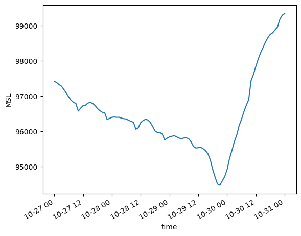
* time (time) datetime64[ns] 2012-10-27 2012-10-27T01:00:00 ... 2012-10-31Call Xarray’s built-in plot method to get a quick look at the time series. Note that we use the Python convention where _ is an object corresponding to the output of the previous line of code.
_.plot()
[<matplotlib.lines.Line2D at 0x14bf340a7f90>]
Perform unit conversions
Convert meters per second to knots, and Pascals to hectoPascals. Both are straightforward with MetPy’s convert_units method.
SLP = SLP.metpy.convert_units('hPa')
U10 = U10.metpy.convert_units('kts')
V10 = V10.metpy.convert_units(‘kts’)
Calculate wind speed from the u- and v- components using MetPy’s diagnostic function, wind_speed.
WSPD = mpcalc.wind_speed(U10,V10)
Perform Split-Apply-Combine
Compute the minimum SLP, and then the maximum wind speed, for all latitude and longitude points … for each time.
SLPmin = SLP.min(dim=['latitude','longitude'])
print(SLPmin)
<xarray.DataArray 'MSL' (time: 97)>
<Quantity([974.2419  973.8619  973.2919  972.83563 971.8862  970.90497 969.8006
 968.8475  968.2631  967.94684 965.77313 966.6287  967.3256  967.4356
 968.0469  968.21185 967.9381  967.3531  966.4956  965.90436 965.45123
 965.2944  963.4031  963.68933 964.0081  964.0881  964.0031  964.02246
 963.75995 963.6031  963.5375  963.1275  962.8831  962.57184 960.6243
 961.0256  962.51685 963.0631  963.44684 963.2375  962.57184 961.40625
 960.12683 959.6794  959.69934 959.225   957.5881  958.0587  958.45435
 958.6281  958.77496 958.45245 958.0956  957.95935 958.1262  958.1744
 957.9187  957.02496 955.7306  955.26874 955.3706  955.47626 955.0706
 954.5612  953.675   951.9212  949.2381  947.01874 945.065   944.7256
 945.9462  947.16376 949.13684 952.26996 954.5325  957.03625 958.9356
 961.5881  963.4531  965.595   967.39746 969.02686 974.4381  976.20874
 978.5281  980.6     982.42    983.84625 985.3775  986.6275  987.57684
 987.9968  988.8612  989.6431  991.87683 993.0156  993.46625], 'hectopascal')>
Coordinates:
  * time     (time) datetime64[ns] 2012-10-27 2012-10-27T01:00:00 ... 2012-10-31
WSPDmax = WSPD.max(dim=['latitude','longitude'])
We’ll take a deeper dive into Xarray’s Split-Apply-Combine implementation in the next notebook.
Here, we’ve effectively reduced the data array down to one dimension (time)!
Create and refine a time series plot of minimum SLP and maximum windspeed over the subsetted region.
Create a meaningful title string.
tl1 = "ERA-5 maximum " + levelStr + " m windspeed (kts) and minimum SLP (hPa)"
tl2 = str('Valid within: '+ domainStr)
title_line = (tl1 + '\n' + tl2 + '\n')
Improve the look of the time-series figure by using Seaborn.
import seaborn as sns
sns.set()
Plot two y-axes; one for SLP, the other for windspeed
fig = plt.figure(figsize=(18,12))
ax1 = plt.subplot(1,1,1)
color = 'tab:red'
ax1.plot(SLP.time,SLPmin,color=color,label = 'Min SLP')

ax1.set_title (title_line,fontsize=14)

ax2 = ax1.twinx()  # instantiate a second axes that shares the same x-axis
color = 'tab:blue'
ax2.plot(WSPD.time,WSPDmax,color=color,label = 'Max Wind');
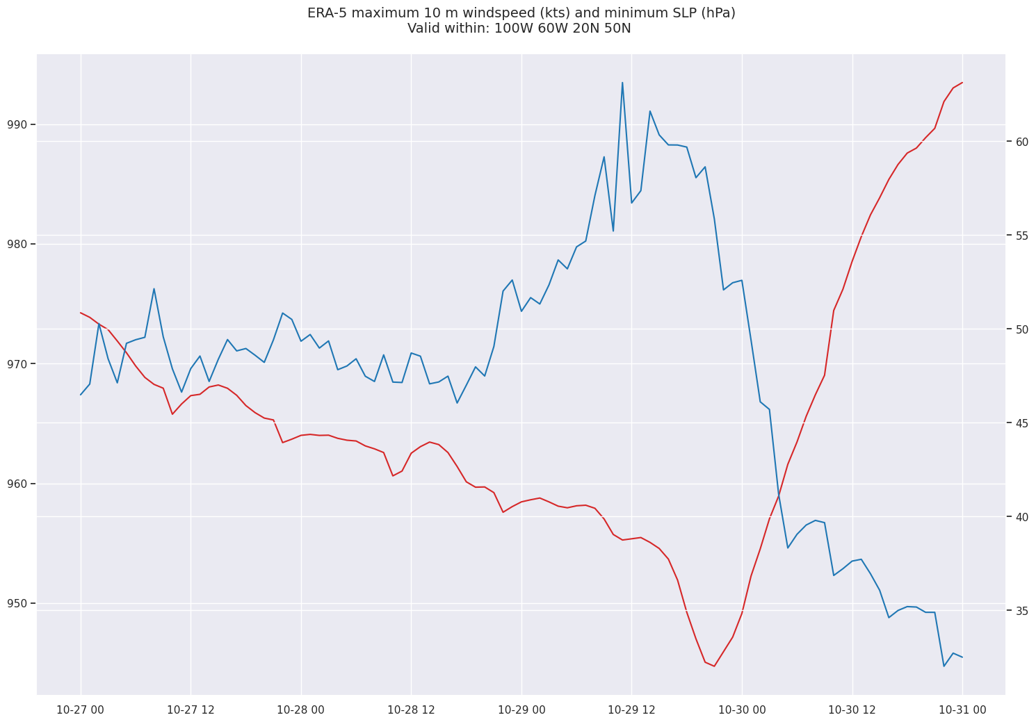
What’s the meaning of tab: in our color definition? It’s one of many color table specifications available in Matplotlib; in this case, tab refers to a color table derived from a commercial dataviz package, Tableau.
That’s not a bad first plot, but much can be done to improve it. Here we use several Matplotlib Axes methods to customize the plot.
Note
Often the best way to learn about these methods (and others) is to browse the relevant documentation at https://matplotlib.org and play around with them. You may be the type who always wants to keep making it look better, but avoid the temptation to keep trying for perfection.
fig = plt.figure(figsize=(18,12),dpi=150)
ax1 = plt.subplot(1,1,1)

# First Axes: SLP
color = 'tab:red'
ax1.plot(SLP.time,SLPmin,color=color,label = 'Min SLP')
ax1.grid(color='black',linewidth=0.5)

ax1.xaxis.set_major_locator(HourLocator(interval=6))
ax1.xaxis.set_minor_locator(HourLocator(interval=1))
dateFmt = DateFormatter('%H')
ax1.xaxis.set_major_formatter(dateFmt)
ax1.set_xlabel('Date/Time (UTC)')
ax1.set_xlim(SLP.time[0],SLP.time[-1])

ax1.set_ylabel('SLP (hPa)',color=color, fontsize=14)
ax1.yaxis.set_minor_locator(MultipleLocator(5))
ax1.tick_params(which='minor', length=6)
ax1.tick_params(which='major',axis='y', labelcolor=color,direction='out', length=6, width=2, colors=color,
               grid_color=color, grid_alpha=0.5)
ax1.tick_params(which='minor', axis = 'y', length=4, color=color)

ax1.set_title (title_line,fontsize=14)

# Second Axes: Windspeed
ax2 = ax1.twinx()  # instantiate a second axes that shares the same x-axis
color = 'tab:blue'
ax2.plot(WSPD.time,WSPDmax,color='tab:blue',label = 'Max Wind')
# Do not draw grid lines (makes plot more readable)
ax2.grid(visible=None)

ax2.set_ylabel('Windspeed (kts)', color=color, fontsize=14)  # we already handled the x-label with ax1
ax2.tick_params(axis='y', labelcolor=color,direction='out', length=6, width=2, colors=color,
               grid_color=color, grid_alpha=0.5) # grid-related specs will be ignored since we are not plotting grid lines for this axes

fig.legend(loc='upper right',frameon=True,bbox_to_anchor=(0.9,1.1), bbox_transform=ax1.transAxes,fontsize=16,shadow=True,edgecolor='purple')
fig.autofmt_xdate(rotation=45);
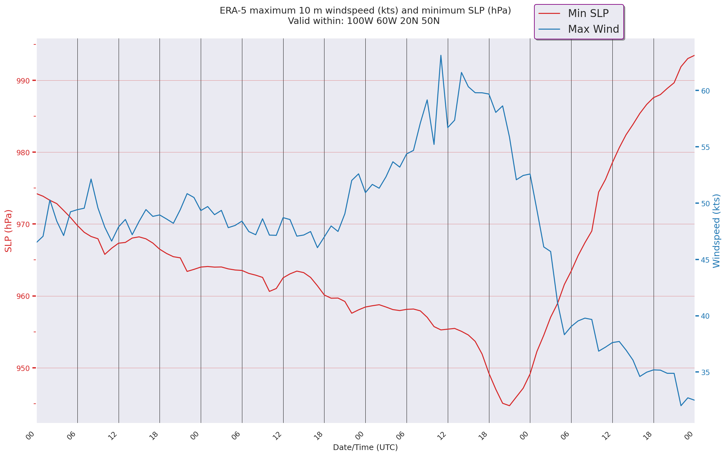
Save our figure to our current directory.
fig.savefig('ERA5_Time_Series.png')