Rasters 2: Overlays
Contents
Rasters 2: Overlays
Overview
Read in a raster file in GeoTIFF format of surface elevation using the Rioxarray package
Explore the attributes of the GeoTIFF file
Plot the GeoTIFF using Matplotlib and Cartopy
Overlay the GeoTIFF on a plot of realtime forecast reflectivity data
Prerequisites
Concepts |
Importance |
Notes |
|---|---|---|
Rasters 1 |
Necessary |
Time to learn: 30 minutes
Be sure to close and shutdown the notebook when finished!
Imports
from datetime import datetime, timedelta
import pandas as pd
import matplotlib.pyplot as plt
import cartopy.crs as ccrs
import cartopy.feature as cfeature
import numpy as np
import xarray as xr

from metpy.plots import USCOUNTIES
from metpy.plots import ctables
import rioxarray as rxr
from matplotlib.colors import BoundaryNorm
from matplotlib.ticker import MaxNLocator
rioxarray library, we've also imported USCOUNTIES from MetPy. This allows for the plotting of US county line boundaries, similar to other Cartopy cartographic features such as states.Additonally, we've imported a set of color tables, also from MetPy.
We've also imported a couple additional methods from Matplotlib, which we'll use to customize the look of our plot when using the
imshow method.
Read in a raster file in GeoTIFF format
Process the topography GeoTIFF file, downloaded from Natural Earth, using the rioxarray package. This package provides an xarray interface while also presenting functionality similar to the rasterio library.
msr = rxr.open_rasterio('/spare11/atm533/data/raster/US_MSR_10M/US_MSR.tif')
Explore the GeoTIFF file. Remember, it’s a TIFF file that is georeferenced.
msr
<xarray.DataArray (band: 1, y: 9493, x: 12578)>
[119402954 values with dtype=uint8]
Coordinates:
  * band         (band) int64 1
  * x            (x) float64 -1.492e+07 -1.492e+07 ... -5.789e+06 -5.788e+06
  * y            (y) float64 7.56e+06 7.559e+06 ... 6.678e+05 6.671e+05
    spatial_ref  int64 0
Attributes:
    AREA_OR_POINT:           Area
    TIFFTAG_DATETIME:        2015:12:30 08:08:29
    TIFFTAG_RESOLUTIONUNIT:  2 (pixels/inch)
    TIFFTAG_SOFTWARE:        Adobe Photoshop CC 2015 (Macintosh)
    TIFFTAG_XRESOLUTION:     350
    TIFFTAG_YRESOLUTION:     350
    scale_factor:            1.0
add_offset: 0.0spatial_ref. This coordinate variable's attributes includes CRS info in what's called well-known text (WKT) format, as well as the Affine transformation parameters. See references at the end of this notebook.
Get the bounding box coordinates of the raster file. We will need to pass them to Matplotlib’s imshow function.
left,bottom,right,top = msr.rio.bounds()
left,bottom,right,top
(-14920200.0, 666726.142827049, -5787726.0672549475, 7560000.0)
These values represent the coordinates, in units specific to the GeoTIFF’s geographic coordinate reference system, of the lower-left and upper-right corners of the raster file.
Get the projection info, which we can later use in Cartopy. A rioxarray dataset object has an attribute called crs for this purpose.
msr.rio.crs
CRS.from_epsg(3857)
Assign this CRS to a Cartopy projection object.
projMSR = ccrs.epsg('3857')
Examine the spatial_ref attribute of this Dataset.
msr.spatial_ref
<xarray.DataArray 'spatial_ref' ()>
array(0)
Coordinates:
    spatial_ref  int64 0
Attributes:
    crs_wkt:       PROJCS["WGS 84 / Pseudo-Mercator",GEOGCS["WGS 84",DATUM["W...
    spatial_ref:   PROJCS["WGS 84 / Pseudo-Mercator",GEOGCS["WGS 84",DATUM["W...
GeoTransform: -14920200.0 726.0672549487241 0.0 7560000.0 0.0 -726.14282...This information makes it possible for GIS applications, such as Cartopy, to transform data that’s represented in one CRS to another.
Select the first (and only) band and redefine the DataArray object, so it only has dimensions of x and y.
msr = msr.sel(band=1)
Determine the min and max values.
msr.min(),msr.max()
(<xarray.DataArray ()>
 array(113, dtype=uint8)
 Coordinates:
     band         int64 1
     spatial_ref  int64 0,
 <xarray.DataArray ()>
 array(249, dtype=uint8)
 Coordinates:
     band         int64 1
     spatial_ref  int64 0)
The next cell will determine how the topography field will be displayed on the figure. These settings work well for this dataset, but obviously must be customized for use with other raster images. This is akin to setting contour fill intervals, but instead of using Matplotlib’s contourf method, we will use imshow, and take advantage of the two Matplotlib methods we imported at the start of the notebook.
# Pick a binning (which is analagous to the # of fill contours, and set a min/max range)
levels = MaxNLocator(nbins=30).tick_values(msr.min(), msr.max()-20)

# Pick the desired colormap, sensible levels, and define a normalization
# instance which takes data values and translates those into levels.
# In this case, we take a color map of 256 discrete colors and normalize them down to 30.
cmap = plt.get_cmap('gist_gray')
norm = BoundaryNorm(levels, ncolors=cmap.N, clip=True)
Examine the levels.
levels
array([112., 116., 120., 124., 128., 132., 136., 140., 144., 148., 152.,
       156., 160., 164., 168., 172., 176., 180., 184., 188., 192., 196.,
       200., 204., 208., 212., 216., 220., 224., 228., 232.])
Plot the GeoTIFF using Matplotlib and Cartopy
Create a region over which we will plot … in this case, centered over NY State.
latN_sub = 45.2
latS_sub = 40.2
lonW_sub = -80.0
lonE_sub = -71.5
cLat_sub = (latN_sub + latS_sub)/2.
cLon_sub = (lonW_sub + lonE_sub )/2.

proj_sub = ccrs.LambertConformal(central_longitude=cLon_sub,
                             central_latitude=cLat_sub,
                             standard_parallels=[cLat_sub])
Plot the GeoTIFF using imshow. Just as we’ve previously transformed data from PlateCarree (lat/lon), here we transform from the Web Mercator projection that the elevation raster file uses.
res = '50m' # Use the medium resolution Natural Earth shapefiles so plotting goes a bit faster than with the highest (10m)
fig = plt.figure(figsize=(18,12))
ax = plt.subplot(1,1,1,projection=proj_sub)
ax.set_extent((lonW_sub,lonE_sub,latS_sub,latN_sub),crs=ccrs.PlateCarree())
ax.set_facecolor(cfeature.COLORS['water'])
ax.add_feature (cfeature.LAND.with_scale(res))
ax.add_feature(cfeature.COASTLINE.with_scale(res))
ax.add_feature (cfeature.LAKES.with_scale(res), alpha = 0.5)
ax.add_feature (cfeature.STATES.with_scale(res))
ax.add_feature(USCOUNTIES,edgecolor='grey', linewidth=1 );
im = ax.imshow(msr,cmap=plt.get_cmap('gist_gray'),
                 alpha=0.4,norm=norm,transform=projMSR, zorder=10)
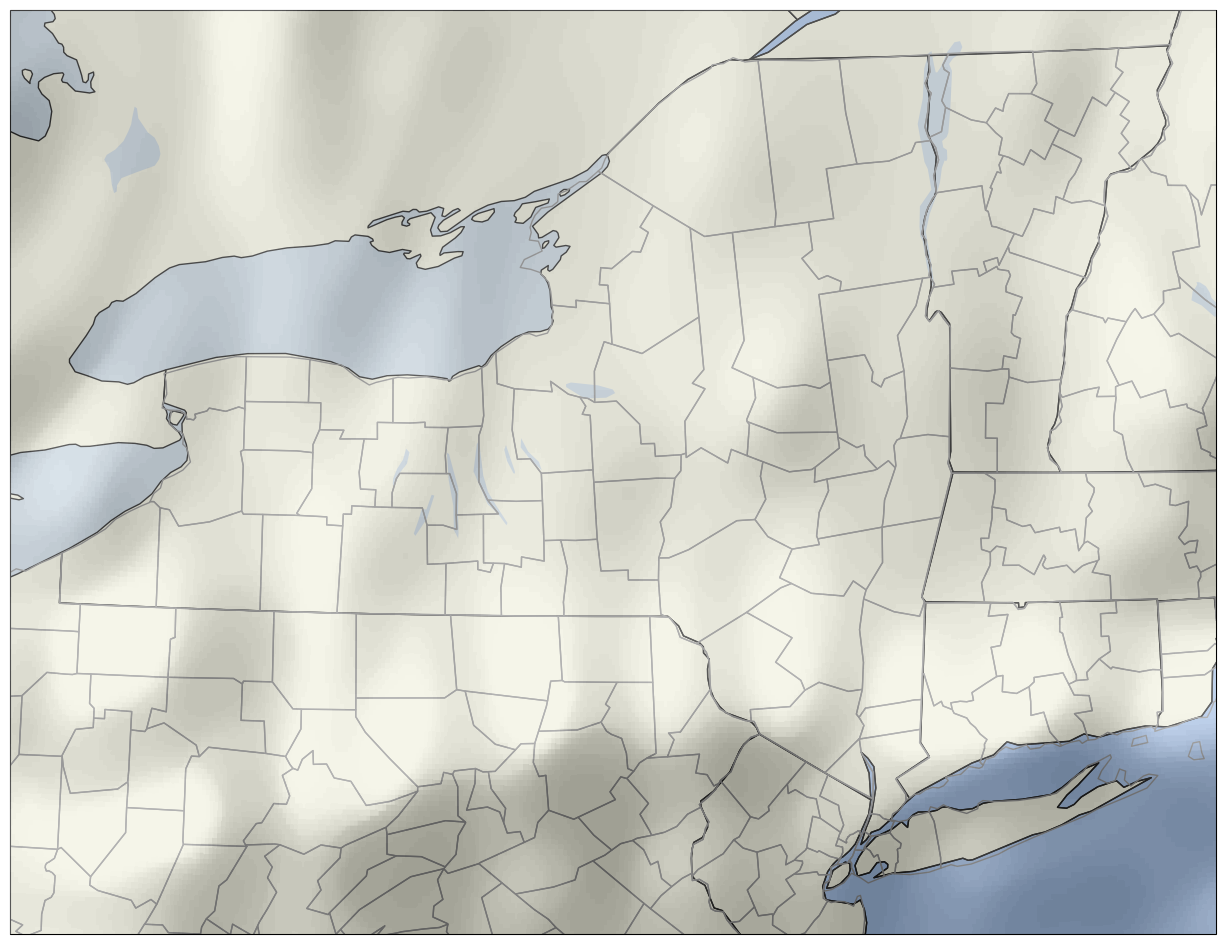
imshow is extent. The default values are not what we want; instead, we use the Bounding Box values that we read in earlier. See the documentation for extent in imshow's documentation.res = '50m'
fig = plt.figure(figsize=(18,12))
ax = plt.subplot(1,1,1,projection=proj_sub)
ax.set_extent((lonW_sub,lonE_sub,latS_sub,latN_sub),crs=ccrs.PlateCarree())
ax.set_facecolor(cfeature.COLORS['water'])
ax.add_feature (cfeature.LAND.with_scale(res))
ax.add_feature(cfeature.COASTLINE.with_scale(res))
ax.add_feature (cfeature.LAKES.with_scale(res), alpha = 0.5)
ax.add_feature (cfeature.STATES.with_scale(res))
ax.add_feature(USCOUNTIES,edgecolor='grey', linewidth=1)
# Pass in the bounding box coordinates as the value for extent
im = ax.imshow(msr, extent = [left,right,bottom,top],cmap=plt.get_cmap('gist_gray'),
alpha=0.4,norm=norm,transform=projMSR);
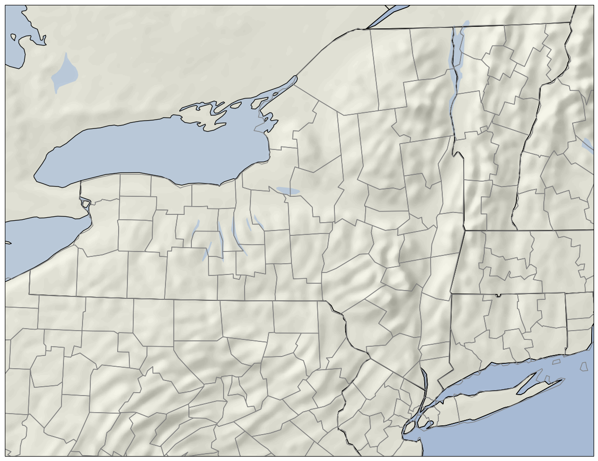
That’s more like it! Now, we can plot maps that include one (or more) GeoTIFF raster images, while also overlaying meteorological data, such as point observations or gridded model output.
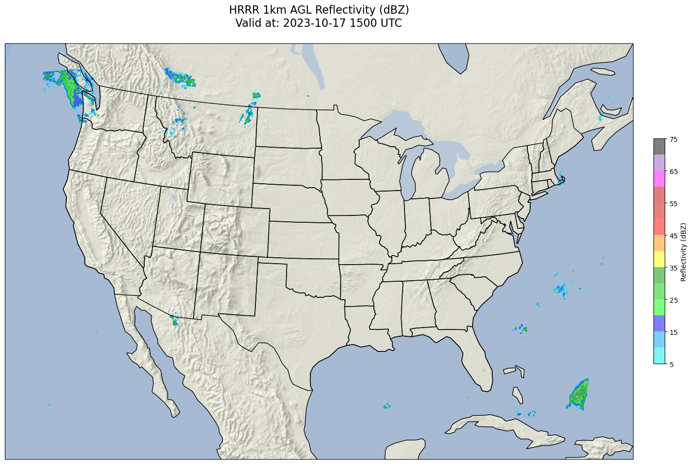
Overlay the GeoTIFF on a plot of realtime forecast reflectivity data
Below, we go through the same steps that we did in the first Raster notebook to gather the latest HRRR model output, but plot filled contours of forecasted 1km above ground level radar reflectivity over the background of topography. We’ll plot over the CONUS.
now = datetime.now()
year = now.year
month = now.month
day = now.day
hour = now.hour
minute = now.minute
print (year, month, day, hour,minute)

if (minute < 45):
    hrDelta = 3
else:
    hrDelta = 2
runTime = now - timedelta(hours=hrDelta)
runTimeStr = runTime.strftime('%Y%m%d %H00 UTC')
modelDate = runTime.strftime('%Y%m%d')
modelHour = runTime.strftime('%H')
modelDay = runTime.strftime('%D')
print (modelDay)
print (modelHour)
print (runTimeStr)
2023 10 17 18 7
10/17/23
15
20231017 1500 UTC
data_url = 'https://thredds.ucar.edu/thredds/dodsC/grib/NCEP/HRRR/CONUS_2p5km/HRRR_CONUS_2p5km_'+ modelDate + '_' + modelHour + '00.grib2'
ds = xr.open_dataset(data_url)
refl = ds.Reflectivity_height_above_ground
refl
<xarray.DataArray 'Reflectivity_height_above_ground' (time: 19,
                                                      height_above_ground1: 1,
                                                      y: 1377, x: 2145)>
[56119635 values with dtype=float32]
Coordinates:
  * x                     (x) float32 -2.763e+03 -2.761e+03 ... 2.682e+03
  * y                     (y) float32 -263.8 -261.3 ... 3.228e+03 3.231e+03
    reftime               datetime64[ns] ...
  * time                  (time) datetime64[ns] 2023-10-17T15:00:00 ... 2023-...
  * height_above_ground1  (height_above_ground1) float32 1e+03
Attributes: (12/13)
    long_name:                       Reflectivity @ Specified height level ab...
    units:                           dB
    abbreviation:                    REFD
    grid_mapping:                    LambertConformal_Projection
    Grib_Variable_Id:                VAR_0-16-195_L103
    Grib2_Parameter:                 [  0  16 195]
    ...                              ...
    Grib2_Parameter_Category:        Forecast Radar Imagery
    Grib2_Parameter_Name:            Reflectivity
    Grib2_Level_Type:                103
    Grib2_Level_Desc:                Specified height level above ground
    Grib2_Generating_Process_Type:   Forecast
Grib2_Statistical_Process_Type: UnknownStatType--1Select the time index (corresponding to the forecast hour; index 0 corresponds to the analysis time) and the (single) height index.
idxTime = 0
idxHght = 0
validTime = refl.time.isel(time = idxTime).values # Returns validTime as a NumPy Datetime 64 object
validTime = pd.Timestamp(validTime) # Converts validTime to a Pandas Timestamp object
timeStr = validTime.strftime("%Y-%m-%d %H%M UTC") # We can now use Datetime's strftime method to create a time string.
tl1 = "HRRR 1km AGL Reflectivity (dBZ)"
tl2 = str('Valid at: '+ timeStr)
title_line = (tl1 + '\n' + tl2 + '\n')
refl = ds.Reflectivity_height_above_ground.isel(time=idxTime, height_above_ground1=idxHght)
Get the projection info from the HRRR Dataset
proj = ds.LambertConformal_Projection

lat1 = proj.latitude_of_projection_origin
lon1 = proj.longitude_of_central_meridian
slat = proj.standard_parallel
projHRRR = ccrs.LambertConformal(central_longitude=lon1,
                             central_latitude=lat1,
                             standard_parallels=[slat])
Use a set of color tables that mimics what the National Weather Services uses for its reflectivity plots.
ref_norm, ref_cmap = ctables.registry.get_with_steps('NWSReflectivity', 5, 5)
refl_range = np.arange(5,80,5)
x = refl.x.metpy.convert_units('m')
y = refl.y.metpy.convert_units('m')
Make the map.
- For speed, choose the coarsest resolution for the cartographic features. It's fine for a larger view such as the CONUS.
- For readability, do not plot county outlines for a regional extent as large as the CONUS
- This step is particularly memory-intensive, since we are reading in two high-resolution rasters (elevation and reflectivity)!
res = '110m'
fig = plt.figure(figsize=(18,12))
ax = plt.subplot(1,1,1,projection=projHRRR)
ax.set_extent((-125,-68,20,52),crs=ccrs.PlateCarree())
ax.set_facecolor(cfeature.COLORS['water'])
ax.add_feature (cfeature.LAND.with_scale(res))
ax.add_feature(cfeature.COASTLINE.with_scale(res))
ax.add_feature (cfeature.LAKES.with_scale(res), alpha = 0.5)
ax.add_feature (cfeature.STATES.with_scale(res))
# Usually avoid plotting counties once the regional extent is large
#ax.add_feature(USCOUNTIES,edgecolor='grey', linewidth=1 );
im = ax.imshow(msr,extent=[left, right, bottom, top],cmap=plt.get_cmap('gist_gray'),
                 alpha=0.4,norm=norm,transform=projMSR)
CF = ax.contourf(x,y,refl,levels=refl_range,cmap=ref_cmap,alpha=0.5,transform=projHRRR)
cbar = plt.colorbar(CF,fraction=0.046, pad=0.03,shrink=0.5)
cbar.ax.tick_params(labelsize=10)
cbar.ax.set_ylabel("Reflectivity (dBZ)",fontsize=10);
title = ax.set_title(title_line,fontsize=16)
Summary
The Rioxarray package allows for raster-specific methods on geo-referenced Xarray objects.
When using
imshowwith Cartopy’s geo-referenced axes in Matplotlib, one must specify theextent, derived from the GeoTIFF’s bounding box.GeoTIFFs can be overlayed with other geo-referenced datasets, such as gridded fields or point observations.
The higher the resolution, the higher the memory usage.
What’s Next?
In the next notebook, we’ll take a look at a multi-band GeoTIFF that is optimized for cloud storage.
References
WKT definitions:
a. From opengeospatial.org
b. From WikipediaAffine transformation defs:
a. From Wikipedia
b. From Univ of Minnesota GIS Course