Contextily 1: Intro
Contents
Contextily 1: Intro
Overview:
Read in the NYS Mesonet sites table with GeoPandas
Plot the NYS Mesonet sites on a map
Use the contextily package to overlay an image as a basemap, served via a remote tile server
Prerequisites
Concepts |
Importance |
Notes |
|---|---|---|
(Geo)Pandas |
Necessary |
|
Cartopy |
Necessary |
Time to learn: 10 minutes
Imports
import cartopy.crs as ccrs
import cartopy.feature as cfeature
import geopandas as gp
import pandas as pd
from metpy.plots import USCOUNTIES
import contextily as ctx
import matplotlib.pyplot as plt
/tmp/ipykernel_4162219/2612810371.py:3: DeprecationWarning: Shapely 2.0 is installed, but because PyGEOS is also installed, GeoPandas still uses PyGEOS by default. However, starting with version 0.14, the default will switch to Shapely. To force to use Shapely 2.0 now, you can either uninstall PyGEOS or set the environment variable USE_PYGEOS=0. You can do this before starting the Python process, or in your code before importing geopandas:

import os
os.environ['USE_PYGEOS'] = '0'
import geopandas

In the next release, GeoPandas will switch to using Shapely by default, even if PyGEOS is installed. If you only have PyGEOS installed to get speed-ups, this switch should be smooth. However, if you are using PyGEOS directly (calling PyGEOS functions on geometries from GeoPandas), this will then stop working and you are encouraged to migrate from PyGEOS to Shapely 2.0 (https://shapely.readthedocs.io/en/latest/migration_pygeos.html).
  import geopandas as gp
Read in the NYS Mesonet sites table with Geopandas
First, open the NYSM sites table using Pandas, as we’ve done before.
nysm_sites = pd.read_csv('/spare11/atm533/data/nysm_sites.csv')
nysm_sites.head()
| stid | number | name | lat | lon | elevation | county | nearest_city | state | distance_from_town [km] | direction_from_town [degrees] | climate_division | climate_division_name | wfo | commissioned | decommissioned | |
|---|---|---|---|---|---|---|---|---|---|---|---|---|---|---|---|---|
| 0 | ADDI | 107 | Addison | 42.04036 | -77.23726 | 507.6140 | Steuben | Addison | NY | 6.9 | S | 1 | Western Plateau | BGM | 2016-08-10 18:15:00 UTC | NaN |
| 1 | ANDE | 111 | Andes | 42.18227 | -74.80139 | 518.2820 | Delaware | Andes | NY | 1.5 | WSW | 2 | Eastern Plateau | BGM | 2016-08-04 15:55:00 UTC | NaN |
| 2 | BATA | 24 | Batavia | 43.01994 | -78.13566 | 276.1200 | Genesee | Batavia | NY | 4.9 | ENE | 9 | Great Lakes | BUF | 2016-02-18 18:40:00 UTC | NaN |
| 3 | BEAC | 76 | Beacon | 41.52875 | -73.94527 | 90.1598 | Dutchess | Beacon | NY | 3.3 | NE | 5 | Hudson Valley | ALY | 2016-08-22 16:45:00 UTC | NaN |
| 4 | BELD | 90 | Belden | 42.22322 | -75.66852 | 470.3700 | Broome | Belden | NY | 2.2 | NNE | 2 | Eastern Plateau | BGM | 2015-11-30 20:20:00 UTC | NaN |
In the Shapefiles Intro notebook, we used Geopandas to read in a shapefile as a Dataframe. Geopandas is not limited to shapefiles; it can also georeference existing Pandas dataframes that contain relevant columns or rows. The NYSM dataframe has latitude and longitude columns; we will pass these in to the GeoDataFrame method which creates the geo-referenced dataframe.
GeoDataFrame requires a column named geometry. Besides polygons and multipolygons, another valid geometry is Points. We thus create a Geometry series using Geopandas' points_from_xy method. This method accepts two series... in this case, the longitude and latitude columns from the NYSM sites dataframe.
gdf = gp.GeoDataFrame(nysm_sites,geometry=gp.points_from_xy(nysm_sites.lon,nysm_sites.lat))
Examine the GeoDataFrame and its geometry column
gdf
| stid | number | name | lat | lon | elevation | county | nearest_city | state | distance_from_town [km] | direction_from_town [degrees] | climate_division | climate_division_name | wfo | commissioned | decommissioned | geometry | |
|---|---|---|---|---|---|---|---|---|---|---|---|---|---|---|---|---|---|
| 0 | ADDI | 107 | Addison | 42.040360 | -77.237260 | 507.6140 | Steuben | Addison | NY | 6.9 | S | 1 | Western Plateau | BGM | 2016-08-10 18:15:00 UTC | NaN | POINT (-77.23726 42.04036) |
| 1 | ANDE | 111 | Andes | 42.182270 | -74.801390 | 518.2820 | Delaware | Andes | NY | 1.5 | WSW | 2 | Eastern Plateau | BGM | 2016-08-04 15:55:00 UTC | NaN | POINT (-74.80139 42.18227) |
| 2 | BATA | 24 | Batavia | 43.019940 | -78.135660 | 276.1200 | Genesee | Batavia | NY | 4.9 | ENE | 9 | Great Lakes | BUF | 2016-02-18 18:40:00 UTC | NaN | POINT (-78.13566 43.01994) |
| 3 | BEAC | 76 | Beacon | 41.528750 | -73.945270 | 90.1598 | Dutchess | Beacon | NY | 3.3 | NE | 5 | Hudson Valley | ALY | 2016-08-22 16:45:00 UTC | NaN | POINT (-73.94527 41.52875) |
| 4 | BELD | 90 | Belden | 42.223220 | -75.668520 | 470.3700 | Broome | Belden | NY | 2.2 | NNE | 2 | Eastern Plateau | BGM | 2015-11-30 20:20:00 UTC | NaN | POINT (-75.66852 42.22322) |
| ... | ... | ... | ... | ... | ... | ... | ... | ... | ... | ... | ... | ... | ... | ... | ... | ... | ... |
| 121 | WFMB | 14 | Whiteface Mountain Base | 44.393236 | -73.858829 | 614.5990 | Essex | Wilmington | NY | 3.5 | W | 3 | Northern Plateau | BTV | 2016-01-29 20:55:00 UTC | NaN | POINT (-73.85883 44.39324) |
| 122 | WGAT | 123 | Woodgate | 43.532408 | -75.158597 | 442.9660 | Oneida | Woodgate | NY | 1.4 | NNW | 3 | Northern Plateau | BGM | 2016-08-29 18:20:00 UTC | NaN | POINT (-75.15860 43.53241) |
| 123 | WHIT | 10 | Whitehall | 43.485073 | -73.423071 | 36.5638 | Washington | Whitehall | NY | 8.0 | S | 7 | Champlain Valley | ALY | 2015-08-26 20:30:00 UTC | NaN | POINT (-73.42307 43.48507) |
| 124 | WOLC | 79 | Wolcott | 43.228680 | -76.842610 | 121.2190 | Wayne | Wolcott | NY | 2.4 | WNW | 9 | Great Lakes | BUF | 2016-03-09 18:10:00 UTC | NaN | POINT (-76.84261 43.22868) |
| 125 | YORK | 99 | York | 42.855040 | -77.847760 | 177.9420 | Livingston | York | NY | 3.6 | ESE | 10 | Central Lakes | BUF | 2016-08-09 17:55:00 UTC | NaN | POINT (-77.84776 42.85504) |
126 rows × 17 columns
As we did in the first Shapefiles notebook, let’s take a look at the geometry attribute of one of the sites.
gdf.loc[gdf.stid == 'VOOR'].geometry
111    POINT (-73.97562 42.65242)
Name: geometry, dtype: geometry
It’s a POINT … whose x- and y- coordinates are the corresponding longitude and latitude in degrees.
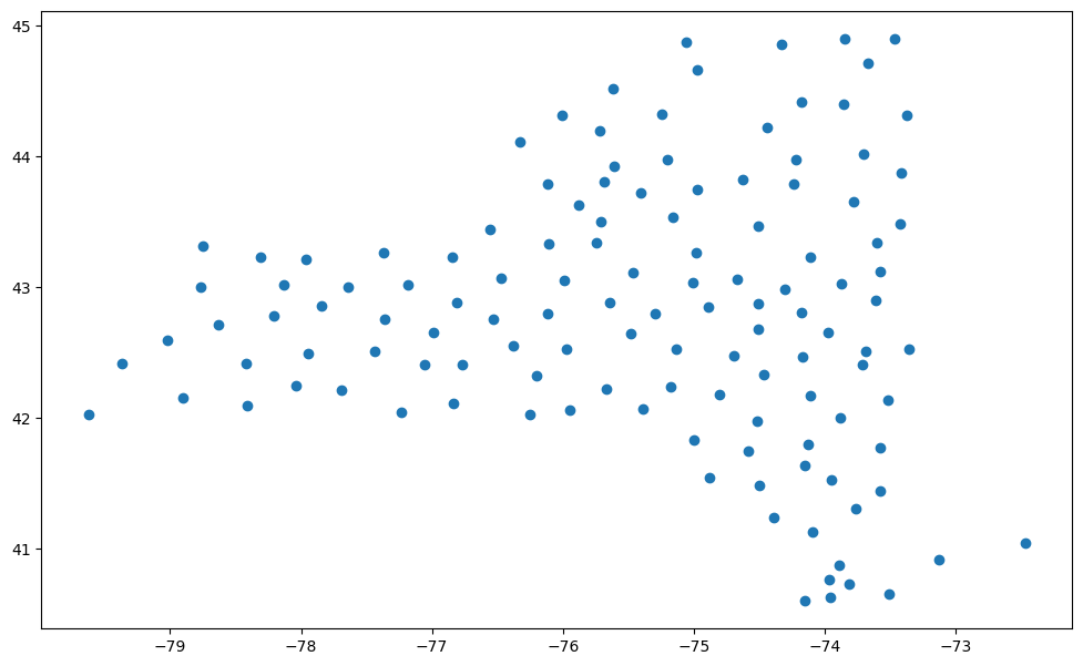
Also as in the previous notebook, we can use Geopandas plot method to get a quick visualization.
gdf.plot(figsize=(12,9));
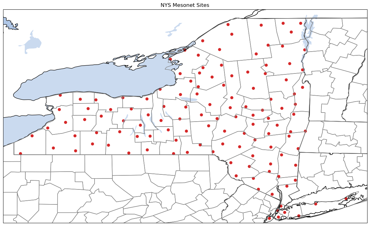
Make a plot using Matplotlib and Cartopy.
To plot the points corresponding to NYS Mesonet sites, we use the same Geopandas plot method, but need to specify the axes. In this case, we first define a set of GeoAxes, as we always do when using Cartopy, and then specify the name of that GeoAxes object as the value for the ax argument.
fig = plt.figure(figsize=(15,10))
ax = plt.axes(projection=ccrs.PlateCarree())

res='10m'
plt.title('NYS Mesonet Sites')
gdf.plot(ax=ax,color='tab:red')

ax.coastlines(resolution=res)
ax.add_feature (cfeature.LAKES.with_scale(res), alpha = 0.5)
ax.add_feature (cfeature.STATES.with_scale(res))
ax.add_feature(USCOUNTIES,edgecolor='grey');
ax.set_extent([-80, -72,40.5,45.2], ccrs.PlateCarree())
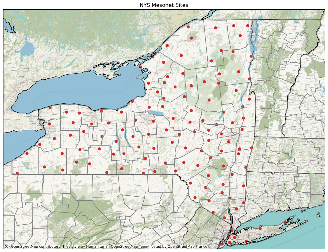
Add a background GeoTIFF raster image.
We’ll use the contextily package’s add_basemap method for that. It will request GeoTIFFs from a remote server that not only provides a source of background maps, but also makes them available at various zoom levels. Depending on how we define the extent of our map, one or more tiles will be downloaded from the remote image server. The default basemap comes from Openstreetmap.
We specify a zoom level here, although if you do not specify one, Contextily will determine an appropriate default value.
fig = plt.figure(figsize=(15,10))
ax = plt.axes(projection=ccrs.epsg('3857'))

res='10m'
plt.title('NYS Mesonet Sites')
gdf.plot(ax=ax,color='tab:red',transform=ccrs.PlateCarree())
ax.coastlines(resolution=res)
ax.add_feature (cfeature.LAKES.with_scale(res), alpha = 0.5)
ax.add_feature (cfeature.STATES.with_scale(res))
ax.add_feature(USCOUNTIES,edgecolor='grey', linewidth=1 );
ax.set_extent([-80, -71.4,40.5,45.2], ccrs.PlateCarree())
ctx.add_basemap(ax,zoom=9,transform=ccrs.epsg('3857'))
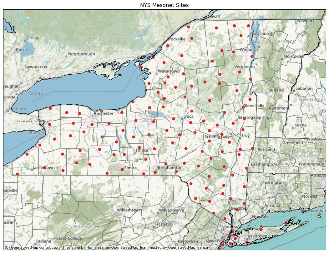
Try a lower zoom value.
fig = plt.figure(figsize=(15,10))
ax = plt.axes(projection=ccrs.epsg('3857'))

res='10m'
plt.title('NYS Mesonet Sites')
gdf.plot(ax=ax,color='tab:red',transform=ccrs.PlateCarree())
ax.coastlines(resolution=res)
ax.add_feature (cfeature.LAKES.with_scale(res), alpha = 0.5)
ax.add_feature (cfeature.STATES.with_scale(res))
ax.add_feature(USCOUNTIES,edgecolor='grey', linewidth=1 );

ax.set_extent([-80, -71.4,40.5,45.2], ccrs.PlateCarree())
ctx.add_basemap(ax,zoom=7,transform=ccrs.epsg('3857'))
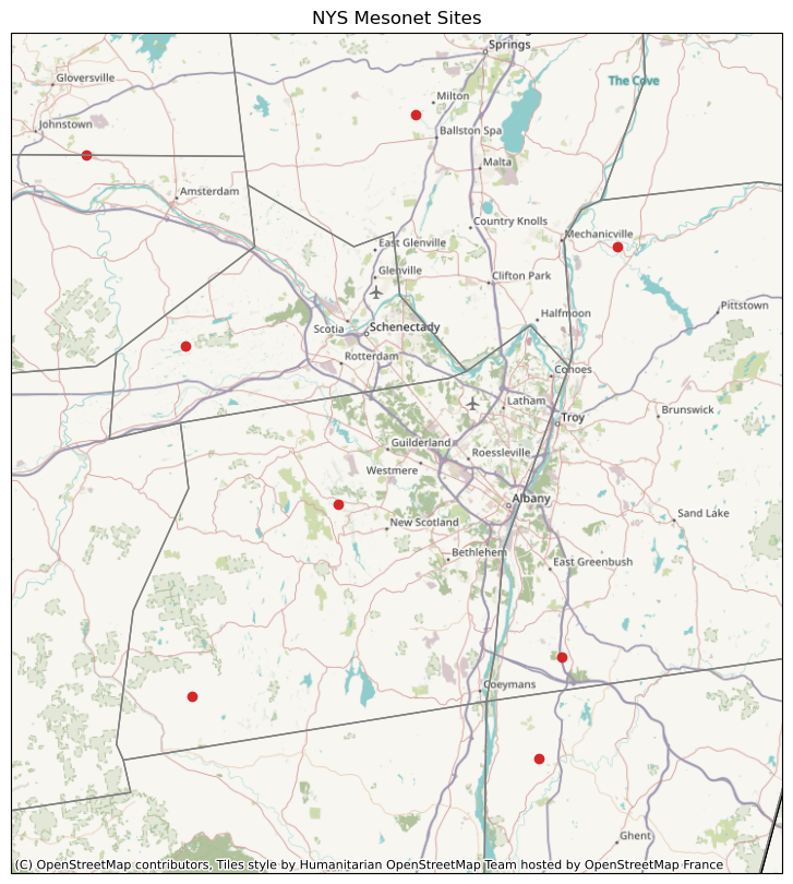
Plot a map whose extent covers just the Greater Capital District.
Do not specify a zoom level. Let contextily’s add_ basemap figure determine the optimum one.
fig = plt.figure(figsize=(15,10))
ax = plt.axes(projection=ccrs.epsg('3857'))

res='10m'
plt.title('NYS Mesonet Sites')
gdf.plot(ax=ax,color='tab:red',transform=ccrs.PlateCarree())
ax.coastlines(resolution=res)

ax.add_feature (cfeature.LAKES.with_scale(res), alpha = 0.5)
ax.add_feature (cfeature.STATES.with_scale(res))
ax.add_feature(USCOUNTIES,edgecolor='grey', linewidth=1 );

ax.set_extent([-74.4, -73.4,42.3,43.1], ccrs.PlateCarree())
ctx.add_basemap(ax)
Summary
Besides shapefiles, Geopandas can geo-reference Pandas dataframes.
The contextily package allows for the plotting of remotely-served basemaps.
These basemap servers support tiling; thus, zooming in or out will reveal greater or less features.
What’s Next?
We’ll explore additional basemaps besides Openstreetmaps … such as high-resolution MODIS satellite composites from NASA.