ERA-5 Data and Graphics Preparation for the Science-on-a-Sphere
Contents
ERA-5 Data and Graphics Preparation for the Science-on-a-Sphere
Overview:
Programmatically request a specific date from the RDA ERA-5 THREDDS repository
Re-arrange the order of the longitudinal dimension in the dataset
Use Cartopy’s
add_cyclic_pointmethod to avoid a blank seam at the datelineCreate 24 hours worth of Science-on-a-Sphere-ready plots
Create a set of labels for each plot
Imports
import xarray as xr
import numpy as np
import pandas as pd
from pandas.tseries.offsets import MonthEnd,MonthBegin
import cartopy.feature as cfeature
import cartopy.crs as ccrs
import cartopy.util as cutil
import requests
from datetime import datetime, timedelta
import warnings
import metpy.calc as mpcalc
from metpy.units import units
import matplotlib.pyplot as plt
ERROR 1: PROJ: proj_create_from_database: Open of /knight/anaconda_aug22/envs/aug22_env/share/proj failed
warnings.simplefilter("ignore")
Programmatically request a specific date from the RDA ERA-5 THREDDS repository
The next several cells set the date/time, creates the URL strings, and retrieves selected grids from RDA.
# Select your date and time here
year = 1978
month = 1
day = 26
hour = 0
While Xarray can create datasets and data arrays from multiple files, via its
open_mfdataset method, this method does not reliably work when reading from a THREDDS server such as RDA's. Therefore, please restrict your temporal range to no more than one calendar day in this notebook.
validTime = datetime(year, month, day, hour)
YYYYMM = validTime.strftime("%Y%m")
YYYYMMDD = validTime.strftime("%Y%m%d")
Among the many tools for time series analysis that Pandas provides are functions to determine the first and last days of a month.
monthEnd = pd.to_datetime(YYYYMM, format='%Y%m') + MonthEnd(0)
mEndStr = monthEnd.strftime('%Y%m%d23')

monthBeg = pd.to_datetime(YYYYMM, format='%Y%m') + MonthBegin(0)
mBegStr = monthBeg.strftime('%Y%m%d00')

dayBegStr = YYYYMMDD + '00'
dayEndStr = YYYYMMDD + '23'

dayBeg = datetime.strptime(dayBegStr, '%Y%m%d%H')
dayEnd = datetime.strptime(dayEndStr, '%Y%m%d%H')
dayBeg, dayEnd
(datetime.datetime(1978, 1, 26, 0, 0), datetime.datetime(1978, 1, 26, 23, 0))
monthBeg, monthEnd
(Timestamp('1978-01-01 00:00:00'), Timestamp('1978-01-31 00:00:00'))
Create the URLs for the various grids.
SfcURL = []
SfcURL.append('https://rda.ucar.edu/thredds/dodsC/files/g/ds633.0/e5.oper.an.')
SfcURL.append(YYYYMM + '/e5.oper.an')
SfcURL.append('.ll025')
SfcURL.append('.' + mBegStr + '_' + mEndStr + '.nc')
print(SfcURL)

PrsURL = []
PrsURL.append('https://rda.ucar.edu/thredds/dodsC/files/g/ds633.0/e5.oper.an.')
PrsURL.append(YYYYMM + '/e5.oper.an')
PrsURL.append('.ll025')
PrsURL.append('.' +  dayBegStr + '_' + dayEndStr + '.nc' )
print(PrsURL)

ds_urlZ = PrsURL[0] + 'pl/' + PrsURL[1] + '.pl.128_129_z' + PrsURL[2] + 'sc' + PrsURL[3]
ds_urlQ = PrsURL[0] + 'pl/' + PrsURL[1] + '.pl.128_133_q' + PrsURL[2] + 'sc' + PrsURL[3]
ds_urlT = PrsURL[0] + 'pl/' + PrsURL[1] + '.pl.128_130_t' + PrsURL[2] + 'sc' + PrsURL[3]
# Notice that U and V use "uv" instead of "sc" in their name!
ds_urlU = PrsURL[0] + 'pl/' + PrsURL[1] + '.pl.128_131_u' + PrsURL[2] + 'uv' + PrsURL[3]
ds_urlV = PrsURL[0] + 'pl/' + PrsURL[1] + '.pl.128_132_v' + PrsURL[2] + 'uv' + PrsURL[3]

ds_urlU10 = SfcURL[0] + 'sfc/' + SfcURL[1] + '.sfc.128_165_10u' + SfcURL[2] + 'sc' + SfcURL[3]
ds_urlV10 = SfcURL[0] + 'sfc/' + SfcURL[1] + '.sfc.128_166_10v' + SfcURL[2] + 'sc' + SfcURL[3]
ds_urlSLP = SfcURL[0] + 'sfc/' + SfcURL[1] + '.sfc.128_151_msl' + SfcURL[2] + 'sc' + SfcURL[3]
['https://rda.ucar.edu/thredds/dodsC/files/g/ds633.0/e5.oper.an.', '197801/e5.oper.an', '.ll025', '.1978010100_1978013123.nc']
['https://rda.ucar.edu/thredds/dodsC/files/g/ds633.0/e5.oper.an.', '197801/e5.oper.an', '.ll025', '.1978012600_1978012623.nc']
Use your RDA credentials to access these individual NetCDF files. You should have previously registered with RDA, and then saved your user id and password in your home directory as .rdarc , with permissions such that only you have read/write access.
#Retrieve login credential for RDA.
from pathlib import Path
HOME = str(Path.home())
credFile = open(HOME+'/.rdarc','r')
userId, pw = credFile.read().split()
Connect to the RDA THREDDS server and point to the files of interest. Here, we’ll comment out the ones we are not interested in but can always uncomment when we want them.
session = requests.Session()
session.auth = (userId, pw)
#storeU10 = xr.backends.PydapDataStore.open(ds_urlU10, session=session)
#storeV10 = xr.backends.PydapDataStore.open(ds_urlV10, session=session)
storeSLP = xr.backends.PydapDataStore.open(ds_urlSLP, session=session)
#storeQ = xr.backends.PydapDataStore.open(ds_urlQ, session=session)
#storeT = xr.backends.PydapDataStore.open(ds_urlT, session=session)
#storeU = xr.backends.PydapDataStore.open(ds_urlU, session=session)
#storeV = xr.backends.PydapDataStore.open(ds_urlV, session=session)
storeZ = xr.backends.PydapDataStore.open(ds_urlZ, session=session)
ds_urlSLP
'https://rda.ucar.edu/thredds/dodsC/files/g/ds633.0/e5.oper.an.sfc/197801/e5.oper.an.sfc.128_151_msl.ll025sc.1978010100_1978013123.nc'
#dsU10 = xr.open_dataset(storeU10)
#dsV10 = xr.open_dataset(storeV10)
dsSLP = xr.open_dataset(storeSLP)
#dsQ   = xr.open_dataset(storeQ)
#dsT   = xr.open_dataset(storeT)
#dsU   = xr.open_dataset(storeU)
#dsV   = xr.open_dataset(storeV)
dsZ   = xr.open_dataset(storeZ)
Examine the datasets
The surface fields span the entire month. Let’s restrict the range so it matches the day of interest.
dsSLP = dsSLP.sel(time=slice(dayBeg,dayEnd))
Create an Xarray DataArray object for SLP and perform unit conversion
SLP = dsSLP['MSL']
SLP = SLP.metpy.convert_units('hPa')
Examine the SLP DataArray
SLP
<xarray.DataArray 'MSL' (time: 24, latitude: 721, longitude: 1440)>
<Quantity([[[1032.5399  1032.5399  1032.5399  ... 1032.5399  1032.5399  1032.5399 ]
  [1032.82    1032.8225  1032.8225  ... 1032.8175  1032.8175  1032.82   ]
  [1033.0275  1033.03    1033.0325  ... 1033.0225  1033.025   1033.025  ]
  ...
  [1009.8475  1009.85    1009.85    ... 1009.83997 1009.84247 1009.845  ]
  [1009.77747 1009.77747 1009.77496 ... 1009.77496 1009.77496 1009.77747]
  [1009.69    1009.69    1009.69    ... 1009.69    1009.69    1009.69   ]]

 [[1031.6238  1031.6238  1031.6238  ... 1031.6238  1031.6238  1031.6238 ]
  [1031.9113  1031.9137  1031.9137  ... 1031.9087  1031.9113  1031.9113 ]
  [1032.1162  1032.1188  1032.1212  ... 1032.1112  1032.1138  1032.1162 ]
  ...
  [1009.84375 1009.84625 1009.84625 ... 1009.83875 1009.83875 1009.84125]
  [1009.78625 1009.78625 1009.78625 ... 1009.78625 1009.78625 1009.78625]
  [1009.70874 1009.70874 1009.70874 ... 1009.70874 1009.70874 1009.70874]]

 [[1031.6018  1031.6018  1031.6018  ... 1031.6018  1031.6018  1031.6018 ]
  [1031.8993  1031.8993  1031.8993  ... 1031.8944  1031.8969  1031.8969 ]
  [1032.1194  1032.1218  1032.1244  ... 1032.1144  1032.1144  1032.1168 ]
  ...
...
  ...
  [1006.08435 1006.08185 1006.07935 ... 1006.08936 1006.08435 1006.08435]
  [1006.33185 1006.32935 1006.32684 ... 1006.33685 1006.33685 1006.33435]
  [1006.89185 1006.89185 1006.89185 ... 1006.89185 1006.89185 1006.89185]]

 [[1021.5062  1021.5062  1021.5062  ... 1021.5062  1021.5062  1021.5062 ]
  [1021.96375 1021.96625 1021.96875 ... 1021.95624 1021.95874 1021.96124]
  [1022.4337  1022.4387  1022.4437  ... 1022.4212  1022.4237  1022.4287 ]
  ...
  [1009.1812  1009.1837  1009.1812  ... 1009.1787  1009.1787  1009.1787 ]
  [1008.89374 1008.89124 1008.89124 ... 1008.89374 1008.89374 1008.89374]
  [1008.97125 1008.97125 1008.97125 ... 1008.97125 1008.97125 1008.97125]]

 [[1021.305   1021.305   1021.305   ... 1021.305   1021.305   1021.305  ]
  [1021.72    1021.72    1021.7225  ... 1021.71246 1021.71497 1021.71747]
  [1022.13995 1022.14496 1022.14996 ... 1022.13    1022.1325  1022.13745]
  ...
  [1009.005   1009.0075  1009.00995 ... 1009.      1009.      1009.     ]
  [1008.6925  1008.6925  1008.6925  ... 1008.6925  1008.6925  1008.6925 ]
  [1008.8075  1008.8075  1008.8075  ... 1008.8075  1008.8075  1008.8075 ]]], 'hectopascal')>
Coordinates:
  * latitude   (latitude) float64 90.0 89.75 89.5 89.25 ... -89.5 -89.75 -90.0
  * longitude  (longitude) float64 0.0 0.25 0.5 0.75 ... 359.0 359.2 359.5 359.8
  * time       (time) datetime64[ns] 1978-01-26 ... 1978-01-26T23:00:00
Attributes:
    long_name:                                          Mean sea level pressure
    short_name:                                         msl
    original_format:                                    WMO GRIB 1 with ECMWF...
    ecmwf_local_table:                                  128
    ecmwf_parameter:                                    151
    minimum_value:                                      93279.19
    maximum_value:                                      106472.31
    grid_specification:                                 0.25 degree x 0.25 de...
    rda_dataset:                                        ds633.0
    rda_dataset_url:                                    https:/rda.ucar.edu/d...
    rda_dataset_doi:                                    DOI: 10.5065/BH6N-5N20
    rda_dataset_group:                                  ERA5 atmospheric surf...
    QuantizeGranularBitGroomNumberOfSignificantDigits:  7
_ChunkSizes: [27, 139, 277]Now examine the geopotential data on isobaric surfaces.
dsZ
<xarray.Dataset>
Dimensions: (time: 24, level: 37, latitude: 721, longitude: 1440)
Coordinates:
* latitude (latitude) float64 90.0 89.75 89.5 89.25 ... -89.5 -89.75 -90.0
* level (level) float64 1.0 2.0 3.0 5.0 7.0 ... 925.0 950.0 975.0 1e+03
* longitude (longitude) float64 0.0 0.25 0.5 0.75 ... 359.0 359.2 359.5 359.8
* time (time) datetime64[ns] 1978-01-26 ... 1978-01-26T23:00:00
Data variables:
Z (time, level, latitude, longitude) float32 ...
utc_date (time) int32 1978012600 1978012601 ... 1978012622 1978012623
Attributes:
DATA_SOURCE: ECMWF: https://cds.climate.copernicus.eu...
NETCDF_CONVERSION: CISL RDA: Conversion from ECMWF GRIB 1 d...
NETCDF_VERSION: 4.8.1
CONVERSION_PLATFORM: Linux r1i3n32 4.12.14-95.51-default #1 S...
CONVERSION_DATE: Sun Jul 3 14:02:30 MDT 2022
Conventions: CF-1.6
NETCDF_COMPRESSION: NCO: Precision-preserving compression to...
history: Sun Jul 3 14:03:04 2022: ncks -4 --ppc ...
NCO: netCDF Operators version 5.0.3 (Homepage...
DODS_EXTRA.Unlimited_Dimension: timeTo reduce the memory footprint for data on isobaric surfaces, let’s request only 6 out of the 37 available levels.
dsZ = dsZ.sel(level = [200,300,500,700,850,1000])
dsZ
<xarray.Dataset>
Dimensions: (time: 24, level: 6, latitude: 721, longitude: 1440)
Coordinates:
* latitude (latitude) float64 90.0 89.75 89.5 89.25 ... -89.5 -89.75 -90.0
* level (level) float64 200.0 300.0 500.0 700.0 850.0 1e+03
* longitude (longitude) float64 0.0 0.25 0.5 0.75 ... 359.0 359.2 359.5 359.8
* time (time) datetime64[ns] 1978-01-26 ... 1978-01-26T23:00:00
Data variables:
Z (time, level, latitude, longitude) float32 ...
utc_date (time) int32 1978012600 1978012601 ... 1978012622 1978012623
Attributes:
DATA_SOURCE: ECMWF: https://cds.climate.copernicus.eu...
NETCDF_CONVERSION: CISL RDA: Conversion from ECMWF GRIB 1 d...
NETCDF_VERSION: 4.8.1
CONVERSION_PLATFORM: Linux r1i3n32 4.12.14-95.51-default #1 S...
CONVERSION_DATE: Sun Jul 3 14:02:30 MDT 2022
Conventions: CF-1.6
NETCDF_COMPRESSION: NCO: Precision-preserving compression to...
history: Sun Jul 3 14:03:04 2022: ncks -4 --ppc ...
NCO: netCDF Operators version 5.0.3 (Homepage...
DODS_EXTRA.Unlimited_Dimension: timeCreate an Xarray DataArray object for Z
Z = dsZ['Z']
Z
<xarray.DataArray 'Z' (time: 24, level: 6, latitude: 721, longitude: 1440)>
[149506560 values with dtype=float32]
Coordinates:
* latitude (latitude) float64 90.0 89.75 89.5 89.25 ... -89.5 -89.75 -90.0
* level (level) float64 200.0 300.0 500.0 700.0 850.0 1e+03
* longitude (longitude) float64 0.0 0.25 0.5 0.75 ... 359.0 359.2 359.5 359.8
* time (time) datetime64[ns] 1978-01-26 ... 1978-01-26T23:00:00
Attributes:
long_name: Geopotential
short_name: z
units: m**2 s**-2
original_format: WMO GRIB 1 with ECMWF...
ecmwf_local_table: 128
ecmwf_parameter: 129
minimum_value: -4556.6367
maximum_value: 494008.56
grid_specification: 0.25 degree x 0.25 de...
rda_dataset: ds633.0
rda_dataset_url: https:/rda.ucar.edu/d...
rda_dataset_doi: DOI: 10.5065/BH6N-5N20
rda_dataset_group: ERA5 atmospheric pres...
QuantizeGranularBitGroomNumberOfSignificantDigits: 7
_ChunkSizes: [1, 37, 721, 1440]Set contour levels for both SLP and Z.
slpLevels = np.arange(864,1080,4)
Choose a particular isobaric surface.
pLevel = 500
Redefine Z so it consists only of the data at the level you just chose.
Z = Z.sel(level=pLevel)
Science-on-a-Sphere requires that projected images, besides using Plate Carree projection, extend from -180 to +180 degrees longitude. The ERA-5 datasets’ longitudinal coordinates start at 0 and go to 360. Define a function that re-sorts datasets (or data arrays) so the longitudinal range begins at the dateline instead of the Greenwich meridian.
def reSortCoords(d):
longitudeName = 'longitude'
d.coords[longitudeName] = (d.coords[longitudeName] + 180) % 360 - 180
d = d.sortby(d[longitudeName])
return d
Z = reSortCoords(Z)
SLP = reSortCoords(SLP)
Examine one of the re-sorted data arrays
SLP
<xarray.DataArray 'MSL' (time: 24, latitude: 721, longitude: 1440)>
<Quantity([[[1032.5399 1032.5399 1032.5399 ... 1032.5399 1032.5399 1032.5399 ]
[1032.28 1032.2775 1032.2775 ... 1032.2825 1032.2825 1032.28 ]
[1031.955 1031.9525 1031.95 ... 1031.9625 1031.96 1031.9575 ]
...
[1008.3675 1008.375 1008.38495 ... 1008.33997 1008.35 1008.3575 ]
[1009.4975 1009.5025 1009.505 ... 1009.485 1009.4875 1009.4925 ]
[1009.69 1009.69 1009.69 ... 1009.69 1009.69 1009.69 ]]
[[1031.6238 1031.6238 1031.6238 ... 1031.6238 1031.6238 1031.6238 ]
[1031.3638 1031.3612 1031.3612 ... 1031.3662 1031.3662 1031.3638 ]
[1031.0387 1031.0363 1031.0337 ... 1031.0437 1031.0413 1031.0387 ]
...
[1008.32874 1008.33875 1008.34625 ... 1008.3012 1008.3087 1008.3187 ]
[1009.4912 1009.4962 1009.5012 ... 1009.47626 1009.4812 1009.4862 ]
[1009.70874 1009.70874 1009.70874 ... 1009.70874 1009.70874 1009.70874]]
[[1031.6018 1031.6018 1031.6018 ... 1031.6018 1031.6018 1031.6018 ]
[1031.3368 1031.3344 1031.3344 ... 1031.3394 1031.3394 1031.3368 ]
[1031.0194 1031.0168 1031.0144 ... 1031.0269 1031.0243 1031.0219 ]
...
...
...
[1005.88434 1005.89685 1005.91187 ... 1005.84186 1005.8569 1005.8693 ]
[1006.70935 1006.71686 1006.72186 ... 1006.68933 1006.69434 1006.70184]
[1006.89185 1006.89185 1006.89185 ... 1006.89185 1006.89185 1006.89185]]
[[1021.5062 1021.5062 1021.5062 ... 1021.5062 1021.5062 1021.5062 ]
[1021.08374 1021.08124 1021.07874 ... 1021.08875 1021.08624 1021.08624]
[1020.7362 1020.7337 1020.7287 ... 1020.7462 1020.7437 1020.7387 ]
...
[1008.1287 1008.13873 1008.14874 ... 1008.09875 1008.1087 1008.1187 ]
[1008.8537 1008.8587 1008.8637 ... 1008.83875 1008.84375 1008.84875]
[1008.97125 1008.97125 1008.97125 ... 1008.97125 1008.97125 1008.97125]]
[[1021.305 1021.305 1021.305 ... 1021.305 1021.305 1021.305 ]
[1020.86 1020.86 1020.8575 ... 1020.8675 1020.865 1020.8625 ]
[1020.3575 1020.3525 1020.3475 ... 1020.37 1020.365 1020.36 ]
...
[1007.8825 1007.89246 1007.90247 ... 1007.855 1007.865 1007.875 ]
[1008.67 1008.675 1008.68 ... 1008.65497 1008.66 1008.665 ]
[1008.8075 1008.8075 1008.8075 ... 1008.8075 1008.8075 1008.8075 ]]], 'hectopascal')>
Coordinates:
* latitude (latitude) float64 90.0 89.75 89.5 89.25 ... -89.5 -89.75 -90.0
* longitude (longitude) float64 -180.0 -179.8 -179.5 ... 179.2 179.5 179.8
* time (time) datetime64[ns] 1978-01-26 ... 1978-01-26T23:00:00
Attributes:
long_name: Mean sea level pressure
short_name: msl
original_format: WMO GRIB 1 with ECMWF...
ecmwf_local_table: 128
ecmwf_parameter: 151
minimum_value: 93279.19
maximum_value: 106472.31
grid_specification: 0.25 degree x 0.25 de...
rda_dataset: ds633.0
rda_dataset_url: https:/rda.ucar.edu/d...
rda_dataset_doi: DOI: 10.5065/BH6N-5N20
rda_dataset_group: ERA5 atmospheric surf...
QuantizeGranularBitGroomNumberOfSignificantDigits: 7
_ChunkSizes: [27, 139, 277]For the purposes of plotting geopotential heights in decameters, choose an appropriate contour interval and range of values … for geopotential heights, a common convention is: from surface up through 700 hPa: 3 dam; above that, 6 dam to 400 and then 9 or 12 dam from 400 and above.
if (pLevel == 1000):
zLevels= np.arange(-90,63, 3)
elif (pLevel == 850):
zLevels = np.arange(60, 183, 3)
elif (pLevel == 700):
zLevels = np.arange(201, 339, 3)
elif (pLevel == 500):
zLevels = np.arange(468, 606, 6)
elif (pLevel == 300):
zLevels = np.arange(765, 1008, 9)
elif (pLevel == 200):
zLevels = np.arange(999, 1305, 9)
#print (U.units)
## Convert wind from m/s to knots; use MetPy to calculate the wind speed.
#UKts = U.metpy.convert_units('knots')
#VKts = V.metpy.convert_units('knots')
## Calculate windspeed.
#wspdKts = calc.wind_speed(U,V).to('knots')
Create objects for the relevant coordinate arrays; in this case, longitude, latitude, and time.
lons, lats, times= SLP.longitude, SLP.latitude, SLP.time
Take a peek at a couple of these coordinate arrays.
lons
<xarray.DataArray 'longitude' (longitude: 1440)> array([-180. , -179.75, -179.5 , ..., 179.25, 179.5 , 179.75]) Coordinates: * longitude (longitude) float64 -180.0 -179.8 -179.5 ... 179.2 179.5 179.8
times
<xarray.DataArray 'time' (time: 24)>
array(['1978-01-26T00:00:00.000000000', '1978-01-26T01:00:00.000000000',
       '1978-01-26T02:00:00.000000000', '1978-01-26T03:00:00.000000000',
       '1978-01-26T04:00:00.000000000', '1978-01-26T05:00:00.000000000',
       '1978-01-26T06:00:00.000000000', '1978-01-26T07:00:00.000000000',
       '1978-01-26T08:00:00.000000000', '1978-01-26T09:00:00.000000000',
       '1978-01-26T10:00:00.000000000', '1978-01-26T11:00:00.000000000',
       '1978-01-26T12:00:00.000000000', '1978-01-26T13:00:00.000000000',
       '1978-01-26T14:00:00.000000000', '1978-01-26T15:00:00.000000000',
       '1978-01-26T16:00:00.000000000', '1978-01-26T17:00:00.000000000',
       '1978-01-26T18:00:00.000000000', '1978-01-26T19:00:00.000000000',
       '1978-01-26T20:00:00.000000000', '1978-01-26T21:00:00.000000000',
       '1978-01-26T22:00:00.000000000', '1978-01-26T23:00:00.000000000'],
      dtype='datetime64[ns]')
Coordinates:
* time (time) datetime64[ns] 1978-01-26 ... 1978-01-26T23:00:00
Attributes:
long_name: time
_ChunkSizes: 1024Create contour plots of SLP and geopotential height.
First, let’s create a single plot, for the first hour of the day. After we have perfected the plot, we will use a for loop to produce a graphic for all 24 hours of our chosen day.
proj_data = ccrs.PlateCarree() # The dataset's x- and y- coordinates are lon-lat
res = '110m'
fig = plt.figure(figsize=(18,12))
ax = plt.subplot(1,1,1,projection=ccrs.PlateCarree())
ax.set_global()
ax.add_feature(cfeature.COASTLINE.with_scale(res))
ax.add_feature(cfeature.STATES.with_scale(res))

# Add the title
valTime = pd.to_datetime(SLP.time[0].values).strftime("%m/%d/%Y at %H UTC")
tl1 = str("ERA-5 SLP and " + str(pLevel) + "hPa Z, " + valTime)
plt.title(tl1,fontsize=16)

# Height (Z) contour fills

# Convert from units of geopotential to height in decameters.
Zdam = mpcalc.geopotential_to_height(Z.isel(time=0)).metpy.convert_units('dam')
CF = ax.contourf(lons,lats,Zdam,levels=zLevels,cmap=plt.get_cmap('viridis'), extend='both')
cbar = fig.colorbar(CF,shrink=0.5)
cbar.set_label(r'Heights (dam)', size='medium')

# SLP contour lines
CL = ax.contour(lons,lats,SLP.isel(time=0),slpLevels,linewidths=1.25,colors='chocolate')
ax.clabel(CL, inline_spacing=0.2, fontsize=8, fmt='%.0f');
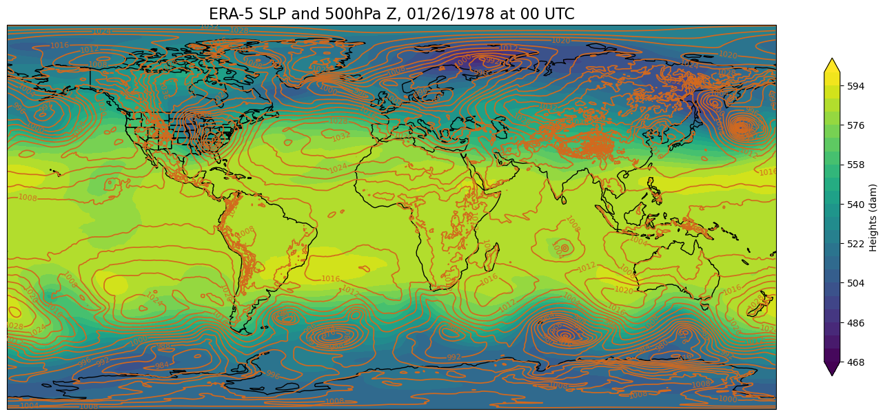
At first glance, this looks good. But let’s re-center the map at the international dateline instead of the Greenwich meridian.
res = '110m'
fig = plt.figure(figsize=(18,12))
ax = plt.subplot(1,1,1,projection=ccrs.PlateCarree(central_longitude=180))
ax.set_global()
ax.add_feature(cfeature.COASTLINE.with_scale(res))
ax.add_feature(cfeature.STATES.with_scale(res))

# Add the title
valTime = pd.to_datetime(SLP.time[0].values).strftime("%m/%d/%Y at %H UTC")
tl1 = str("ERA-5 SLP and " + str(pLevel) + "hPa Z, " + valTime)
plt.title(tl1,fontsize=16)

# Height (Z) contour fills

# Convert from units of geopotential to height in decameters.
Zdam = mpcalc.geopotential_to_height(Z.isel(time=0)).metpy.convert_units('dam')
CF = ax.contourf(lons,lats,Zdam,levels=zLevels,cmap=plt.get_cmap('viridis'), extend='both')
cbar = fig.colorbar(CF,shrink=0.5)
cbar.set_label(r'Heights (dam)', size='medium')

# SLP contour lines
CL = ax.contour(lons,lats,SLP.isel(time=0),slpLevels,linewidths=1.25,colors='chocolate')
ax.clabel(CL, inline_spacing=0.2, fontsize=8, fmt='%.0f');
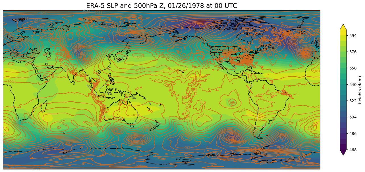
That still looks good, right? Let’s now try plotting on an orthographic projection, somewhat akin to how it would look on the sphere.
res = '110m'
fig = plt.figure(figsize=(18,12))
ax = plt.subplot(1,1,1,projection=ccrs.Orthographic(central_longitude=180))
ax.set_global()
ax.add_feature(cfeature.COASTLINE.with_scale(res))
ax.add_feature(cfeature.STATES.with_scale(res))

# Add the title
valTime = pd.to_datetime(SLP.time[0].values).strftime("%m/%d/%Y at %H UTC")
tl1 = str("ERA-5 SLP and " + str(pLevel) + "hPa Z, " + valTime)
plt.title(tl1,fontsize=16)

# Height (Z) contour fills

# Convert from units of geopotential to height in decameters.
Zdam = mpcalc.geopotential_to_height(Z.isel(time=0)).metpy.convert_units('dam')
CF = ax.contourf(lons,lats,Zdam,levels=zLevels,cmap=plt.get_cmap('viridis'), extend='both', transform=proj_data) # We need the transform argument now
cbar = fig.colorbar(CF,shrink=0.5)
cbar.set_label(r'Heights (dam)', size='medium')

# SLP contour lines
CL = ax.contour(lons,lats,SLP.isel(time=0),slpLevels,linewidths=1.25,colors='chocolate', transform=proj_data)
ax.clabel(CL, inline_spacing=0.2, fontsize=8, fmt='%.0f');
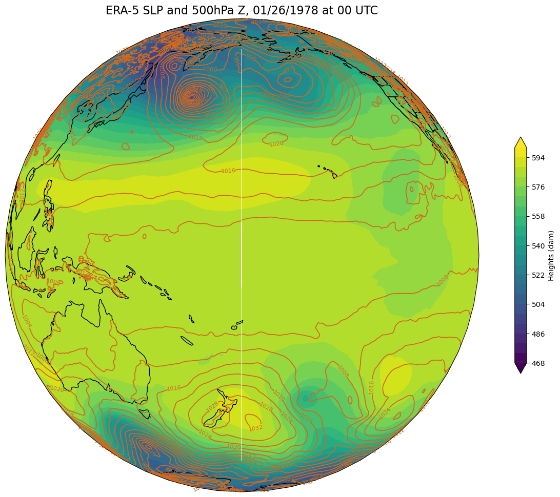
There “seams” to be a problem close to the dateline. This is because the longitude ends at 179.75 E … leaving a gap between 179.75 and 180 degrees. Fortunately, Cartopy includes the add_cyclic_point method in its utilities class to deal with this rather common phenomenon in global gridded datasets.
res = '110m'
fig = plt.figure(figsize=(18,12))
ax = plt.subplot(1,1,1,projection=ccrs.Orthographic(central_longitude=180))
ax.set_global()
ax.add_feature(cfeature.COASTLINE.with_scale(res))
ax.add_feature(cfeature.STATES.with_scale(res))

# Add the title
valTime = pd.to_datetime(SLP.time[0].values).strftime("%m/%d/%Y at %H UTC")
tl1 = str("ERA-5 SLP and " + str(pLevel) + "hPa Z, " + valTime)
plt.title(tl1,fontsize=16)

# Convert from units of geopotential to height in decameters.
Zdam = mpcalc.geopotential_to_height(Z.isel(time=0)).metpy.convert_units('dam')

# add cyclic points to data and longitudes
# latitudes are unchanged in 1-dimension
SLP2d, clons= cutil.add_cyclic_point(SLP.isel(time=0), lons)
z2d, clons = cutil.add_cyclic_point(Zdam, lons)

# Height (Z) contour fills


CF = ax.contourf(clons,lats,z2d,levels=zLevels,cmap=plt.get_cmap('viridis'), extend='both', transform=proj_data) # We need the transform argument now
cbar = fig.colorbar(CF,shrink=0.5)
cbar.set_label(r'Heights (dam)', size='medium')

# SLP contour lines
CL = ax.contour(clons,lats,SLP2d,slpLevels,linewidths=1.25,colors='chocolate', transform=proj_data)
ax.clabel(CL, inline_spacing=0.2, fontsize=8, fmt='%.0f');

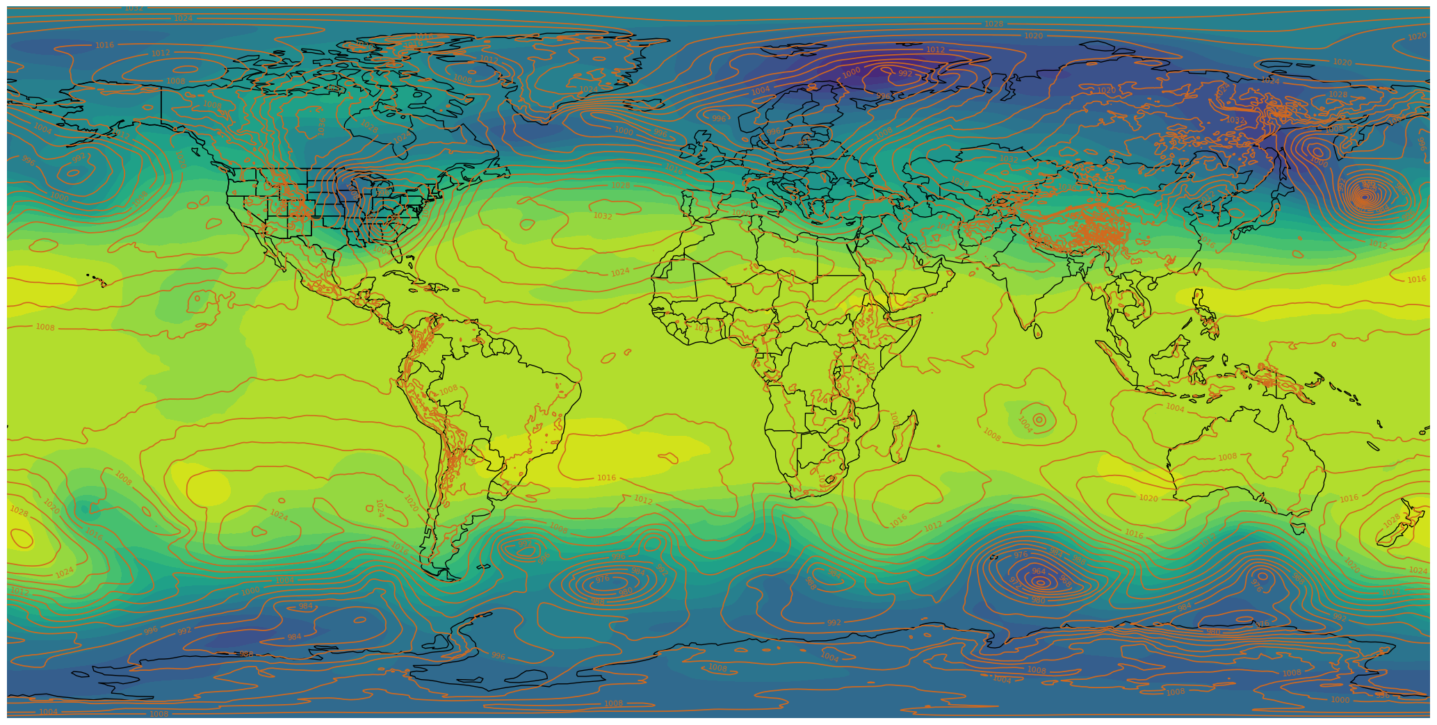
The white seam is gone … now let’s go back to the PlateCarree projection, centered once again at its default value of 0 degrees.
Additionally, the sphere expects its graphics to have a resolution of 2048x1024.
Finally, by default, Matplotlib includes a border frame around each
Axes. We don't want that included on the sphere-projected graphic either.res = '110m'
dpi = 100
fig = plt.figure(figsize=(2048/dpi, 1024/dpi))
ax = plt.subplot(1,1,1,projection=ccrs.PlateCarree(), frameon=False)
ax.set_global()
ax.add_feature(cfeature.COASTLINE.with_scale(res))
ax.add_feature(cfeature.BORDERS.with_scale(res))
ax.add_feature(cfeature.STATES.with_scale(res))
# Convert from units of geopotential to height in decameters.
Zdam = mpcalc.geopotential_to_height(Z.isel(time=0)).metpy.convert_units('dam')
# add cyclic points to data and longitudes
# latitudes are unchanged in 1-dimension
SLP2d, clons= cutil.add_cyclic_point(SLP.isel(time=0), lons)
z2d, clons = cutil.add_cyclic_point(Zdam, lons)
# Height (Z) contour fills
# Note we don't need the transform argument since the map/data projections are the same, but we'll leave it in
CF = ax.contourf(clons,lats,z2d,levels=zLevels,cmap=plt.get_cmap('viridis'), extend='both', transform=proj_data)
# SLP contour lines
CL = ax.contour(clons,lats,SLP2d,slpLevels,linewidths=1.25,colors='chocolate', transform=proj_data)
ax.clabel(CL, inline_spacing=0.2, fontsize=8, fmt='%.0f')
fig.tight_layout(pad=.01)
fig.savefig("test1.png")
Define a function to create the plot for each hour.
The function accepts the hour and a DataArray as its arguments.
def make_sos_map (i, z):
    res = '110m'
    dpi = 100
    fig = plt.figure(figsize=(2048/dpi, 1024/dpi))
    ax = plt.subplot(1,1,1,projection=ccrs.PlateCarree(), frameon=False)
    ax.set_global()
    ax.add_feature(cfeature.COASTLINE.with_scale(res))
    ax.add_feature(cfeature.BORDERS.with_scale(res))
    ax.add_feature(cfeature.STATES.with_scale(res))

    # add cyclic points to data and longitudes
    # latitudes are unchanged in 1-dimension
    SLP2d, clons= cutil.add_cyclic_point(SLP.isel(time=i), lons)
    z2d, clons = cutil.add_cyclic_point(z, lons)

    # Height (Z) contour fills

    CF = ax.contourf(clons,lats,z2d,levels=zLevels,cmap=plt.get_cmap('viridis'), extend='both')

    # SLP contour lines
    CL = ax.contour(clons,lats,SLP2d,slpLevels,linewidths=1.25,colors='chocolate', transform=proj_data)
    ax.clabel(CL, inline_spacing=0.2, fontsize=8, fmt='%.0f')
    fig.tight_layout(pad=.01)
    frameNum = str(i).zfill(2)
    fig.savefig('ERA5_780126' + frameNum  + '.png')
    plt.close()
Open a handle to a text file that will contain each plot’s title.
fileName = '500Z_SLP.txt' # Modify the filename to fit the context of your plot.
Execute the for loop
Loop over the 24 hours and create each hour’s graphic and write the title line to the text file. We will also convert the geopotential grid into height in decameters.
inc to 1 so all hours are processed. fileObject = open(fileName, 'w')
startHr = 0
endHr = 24
inc = 12 #
for time in range(startHr, endHr, inc):
# Perform any unit conversions appropriate for your scalar quantities. In this example,
# we convert geopotential to geopotential height in decameters.
z = mpcalc.geopotential_to_height(Z.isel(time=time)).metpy.convert_units('dam')
make_sos_map(time,z)
# Construct the title string and write it to the file
valTime = pd.to_datetime(times[time].values).strftime("%m/%d/%Y %H UTC")
tl1 = str("SLP & " + str(pLevel) + " hPa Z " + valTime + "\n") # \n is the newline character
fileObject.write(tl1)
print(tl1)
# Close the text file
fileObject.close()
SLP & 500 hPa Z 01/26/1978 00 UTC
SLP & 500 hPa Z 01/26/1978 12 UTC
Summary
We now have a means of creating graphics and corresponding title strings that we can upload and ultimately visualize on our Science-on-a-Sphere.
What’s Next?
We will create a SoS-friendly color bar for any products that use a contour fill. After that, we will have everything we need for our SoS visualization, and just need to learn how to make it ready for upload to the SoS computer.