Xarray and ERA5
Contents
Xarray and ERA5
Overview:
Programmatically request a specific date from the RDA ERA-5 THREDDS repository
Create a time loop and create products of interest for each time in the loop
Imports
import xarray as xr
import numpy as np
import pandas as pd
from pandas.tseries.offsets import MonthEnd,MonthBegin
import cartopy.feature as cfeature
import cartopy.crs as ccrs
import requests
from datetime import datetime, timedelta
import warnings
import metpy.calc as mpcalc
from metpy.units import units
import matplotlib.pyplot as plt
ERROR 1: PROJ: proj_create_from_database: Open of /knight/anaconda_aug22/envs/aug22_env/share/proj failed
Programmatically request a specific date from the RDA ERA-5 THREDDS repository
The next several cells set the date/time, creates the URL strings, and retrieves selected grids from RDA.
For this notebook, we choose the “Cleveland Superbomb” case of January 26, 1978.
# Select your date and time here
year = 1978
month = 1
day = 26
hour = 0
While Xarray can create datasets and data arrays from multiple files, via its
open_mfdataset method, this method does not reliably work when reading from a THREDDS server such as RDA's. Therefore, please restrict your temporal range to no more than one calendar day in this notebook.
validTime = datetime(year, month, day, hour)
YYYYMM = validTime.strftime("%Y%m")
YYYYMMDD = validTime.strftime("%Y%m%d")
Among the many tools for time series analysis that Pandas provides are functions to determine the first and last days of a month.
monthEnd = pd.to_datetime(YYYYMM, format='%Y%m') + MonthEnd(0)
mEndStr = monthEnd.strftime('%Y%m%d23')

monthBeg = pd.to_datetime(YYYYMM, format='%Y%m') + MonthBegin(0)
mBegStr = monthBeg.strftime('%Y%m%d00')

dayBegStr = YYYYMMDD + '00'
dayEndStr = YYYYMMDD + '23'

dayBeg = datetime.strptime(dayBegStr, '%Y%m%d%H')
dayEnd = datetime.strptime(dayEndStr, '%Y%m%d%H')
dayBeg, dayEnd
(datetime.datetime(1978, 1, 26, 0, 0), datetime.datetime(1978, 1, 26, 23, 0))
monthBeg, monthEnd
(Timestamp('1978-01-01 00:00:00'), Timestamp('1978-01-31 00:00:00'))
Create the URLs for the various grids.
SfcURL = []
SfcURL.append('https://rda.ucar.edu/thredds/dodsC/files/g/ds633.0/e5.oper.an.')
SfcURL.append(YYYYMM + '/e5.oper.an')
SfcURL.append('.ll025')
SfcURL.append('.' + mBegStr + '_' + mEndStr + '.nc')
print(SfcURL)

PrsURL = []
PrsURL.append('https://rda.ucar.edu/thredds/dodsC/files/g/ds633.0/e5.oper.an.')
PrsURL.append(YYYYMM + '/e5.oper.an')
PrsURL.append('.ll025')
PrsURL.append('.' +  dayBegStr + '_' + dayEndStr + '.nc' )
print(PrsURL)

ds_urlZ = PrsURL[0] + 'pl/' + PrsURL[1] + '.pl.128_129_z' + PrsURL[2] + 'sc' + PrsURL[3]
ds_urlQ = PrsURL[0] + 'pl/' + PrsURL[1] + '.pl.128_133_q' + PrsURL[2] + 'sc' + PrsURL[3]
ds_urlT = PrsURL[0] + 'pl/' + PrsURL[1] + '.pl.128_130_t' + PrsURL[2] + 'sc' + PrsURL[3]
# Notice that U and V use "uv" instead of "sc" in their name!
ds_urlU = PrsURL[0] + 'pl/' + PrsURL[1] + '.pl.128_131_u' + PrsURL[2] + 'uv' + PrsURL[3]
ds_urlV = PrsURL[0] + 'pl/' + PrsURL[1] + '.pl.128_132_v' + PrsURL[2] + 'uv' + PrsURL[3]

ds_urlU10 = SfcURL[0] + 'sfc/' + SfcURL[1] + '.sfc.128_165_10u' + SfcURL[2] + 'sc' + SfcURL[3]
ds_urlV10 = SfcURL[0] + 'sfc/' + SfcURL[1] + '.sfc.128_166_10v' + SfcURL[2] + 'sc' + SfcURL[3]
ds_urlSLP = SfcURL[0] + 'sfc/' + SfcURL[1] + '.sfc.128_151_msl' + SfcURL[2] + 'sc' + SfcURL[3]
['https://rda.ucar.edu/thredds/dodsC/files/g/ds633.0/e5.oper.an.', '197801/e5.oper.an', '.ll025', '.1978010100_1978013123.nc']
['https://rda.ucar.edu/thredds/dodsC/files/g/ds633.0/e5.oper.an.', '197801/e5.oper.an', '.ll025', '.1978012600_1978012623.nc']
Use your RDA credentials to access these individual NetCDF files. You should have previously registered with RDA, and then saved your user id and password in your home directory as .rdarc , with permissions such that only you have read/write access.
#Retrieve login credential for RDA.
from pathlib import Path
HOME = str(Path.home())
credFile = open(HOME+'/.rdarc','r')
userId, pw = credFile.read().split()
Connect to the RDA THREDDS server and point to the files of interest. Here, we’ll comment out the ones we are not interested in but can always uncomment when we want them.
session = requests.Session()
session.auth = (userId, pw)
#storeU10 = xr.backends.PydapDataStore.open(ds_urlU10, session=session)
#storeV10 = xr.backends.PydapDataStore.open(ds_urlV10, session=session)
storeSLP = xr.backends.PydapDataStore.open(ds_urlSLP, session=session)
#storeQ = xr.backends.PydapDataStore.open(ds_urlQ, session=session)
#storeT = xr.backends.PydapDataStore.open(ds_urlT, session=session)
#storeU = xr.backends.PydapDataStore.open(ds_urlU, session=session)
#storeV = xr.backends.PydapDataStore.open(ds_urlV, session=session)
storeZ = xr.backends.PydapDataStore.open(ds_urlZ, session=session)
ds_urlSLP
'https://rda.ucar.edu/thredds/dodsC/files/g/ds633.0/e5.oper.an.sfc/197801/e5.oper.an.sfc.128_151_msl.ll025sc.1978010100_1978013123.nc'
#dsU10 = xr.open_dataset(storeU10)
#dsV10 = xr.open_dataset(storeV10)
dsSLP = xr.open_dataset(storeSLP)
#dsQ   = xr.open_dataset(storeQ)
#dsT   = xr.open_dataset(storeT)
#dsU   = xr.open_dataset(storeU)
#dsV   = xr.open_dataset(storeV)
dsZ   = xr.open_dataset(storeZ)
Examine the datasets
The surface fields span the entire month. Let’s restrict the range so it matches the day of interest.
dsSLP = dsSLP.sel(time=slice(dayBeg,dayEnd))
dsSLP
<xarray.Dataset>
Dimensions:    (time: 24, latitude: 721, longitude: 1440)
Coordinates:
  * latitude   (latitude) float64 90.0 89.75 89.5 89.25 ... -89.5 -89.75 -90.0
  * longitude  (longitude) float64 0.0 0.25 0.5 0.75 ... 359.0 359.2 359.5 359.8
  * time       (time) datetime64[ns] 1978-01-26 ... 1978-01-26T23:00:00
Data variables:
    MSL        (time, latitude, longitude) float32 ...
    utc_date   (time) int32 1978012600 1978012601 ... 1978012622 1978012623
Attributes:
    DATA_SOURCE:                     ECMWF: https://cds.climate.copernicus.eu...
    NETCDF_CONVERSION:               CISL RDA: Conversion from ECMWF GRIB1 da...
    NETCDF_VERSION:                  4.8.1
    CONVERSION_PLATFORM:             Linux r1i3n33 4.12.14-95.51-default #1 S...
    CONVERSION_DATE:                 Sun Jul  3 15:10:46 MDT 2022
    Conventions:                     CF-1.6
    NETCDF_COMPRESSION:              NCO: Precision-preserving compression to...
    history:                         Sun Jul  3 15:11:09 2022: ncks -4 --ppc ...
    NCO:                             netCDF Operators version 5.0.3 (Homepage...
DODS_EXTRA.Unlimited_Dimension: timeCreate an Xarray DataArray object for SLP and perform unit conversion
SLP = dsSLP['MSL']
SLP = SLP.metpy.convert_units('hPa')
Now examine the geopotential data on isobaric surfaces.
dsZ
<xarray.Dataset>
Dimensions: (time: 24, level: 37, latitude: 721, longitude: 1440)
Coordinates:
* latitude (latitude) float64 90.0 89.75 89.5 89.25 ... -89.5 -89.75 -90.0
* level (level) float64 1.0 2.0 3.0 5.0 7.0 ... 925.0 950.0 975.0 1e+03
* longitude (longitude) float64 0.0 0.25 0.5 0.75 ... 359.0 359.2 359.5 359.8
* time (time) datetime64[ns] 1978-01-26 ... 1978-01-26T23:00:00
Data variables:
Z (time, level, latitude, longitude) float32 ...
utc_date (time) int32 1978012600 1978012601 ... 1978012622 1978012623
Attributes:
DATA_SOURCE: ECMWF: https://cds.climate.copernicus.eu...
NETCDF_CONVERSION: CISL RDA: Conversion from ECMWF GRIB 1 d...
NETCDF_VERSION: 4.8.1
CONVERSION_PLATFORM: Linux r1i3n32 4.12.14-95.51-default #1 S...
CONVERSION_DATE: Sun Jul 3 14:02:30 MDT 2022
Conventions: CF-1.6
NETCDF_COMPRESSION: NCO: Precision-preserving compression to...
history: Sun Jul 3 14:03:04 2022: ncks -4 --ppc ...
NCO: netCDF Operators version 5.0.3 (Homepage...
DODS_EXTRA.Unlimited_Dimension: timeTo reduce the memory footprint for data on isobaric surfaces, let’s request only 6 out of the 37 available levels.
dsZ = dsZ.sel(level = [200,300,500,700,850,1000])
Z = dsZ['Z']
Z
<xarray.DataArray 'Z' (time: 24, level: 6, latitude: 721, longitude: 1440)>
[149506560 values with dtype=float32]
Coordinates:
* latitude (latitude) float64 90.0 89.75 89.5 89.25 ... -89.5 -89.75 -90.0
* level (level) float64 200.0 300.0 500.0 700.0 850.0 1e+03
* longitude (longitude) float64 0.0 0.25 0.5 0.75 ... 359.0 359.2 359.5 359.8
* time (time) datetime64[ns] 1978-01-26 ... 1978-01-26T23:00:00
Attributes:
long_name: Geopotential
short_name: z
units: m**2 s**-2
original_format: WMO GRIB 1 with ECMWF...
ecmwf_local_table: 128
ecmwf_parameter: 129
minimum_value: -4556.6367
maximum_value: 494008.56
grid_specification: 0.25 degree x 0.25 de...
rda_dataset: ds633.0
rda_dataset_url: https:/rda.ucar.edu/d...
rda_dataset_doi: DOI: 10.5065/BH6N-5N20
rda_dataset_group: ERA5 atmospheric pres...
QuantizeGranularBitGroomNumberOfSignificantDigits: 7
_ChunkSizes: [1, 37, 721, 1440]Set contour levels for both SLP and Z.
slpLevels = np.arange(900,1080,4)
Choose a particular isobaric surface.
pLevel = 500
Redefine Z so it consists only of the data at the level you just chose.
Z = Z.sel(level=pLevel)
For the purposes of plotting geopotential heights in decameters, choose an appropriate contour interval and range of values … for geopotential heights, a common convention is: from surface up through 700 hPa: 3 dam; above that, 6 dam to 400 and then 9 or 12 dam from 400 and above.
if (pLevel == 1000):
zLevels= np.arange(-90,63, 3)
elif (pLevel == 850):
zLevels = np.arange(60, 183, 3)
elif (pLevel == 700):
zLevels = np.arange(201, 339, 3)
elif (pLevel == 500):
zLevels = np.arange(468, 606, 6)
elif (pLevel == 300):
zLevels = np.arange(765, 1008, 9)
elif (pLevel == 200):
zLevels = np.arange(999, 1305, 9)
#print (U.units)
## Convert wind from m/s to knots; use MetPy to calculate the wind speed.
#UKts = U.metpy.convert_units('knots')
#VKts = V.metpy.convert_units('knots')
## Calculate windspeed.
#wspdKts = calc.wind_speed(U,V).to('knots')
Create objects for the relevant coordinate arrays; in this case, longitude, latitude, and time.
lons, lats, times= SLP.longitude, SLP.latitude, SLP.time
Take a peek at a couple of these coordinate arrays.
lons
<xarray.DataArray 'longitude' (longitude: 1440)>
array([0.0000e+00, 2.5000e-01, 5.0000e-01, ..., 3.5925e+02, 3.5950e+02,
       3.5975e+02])
Coordinates:
* longitude (longitude) float64 0.0 0.25 0.5 0.75 ... 359.0 359.2 359.5 359.8
Attributes:
long_name: longitude
short_name: lon
units: degrees_east
_ChunkSizes: 1440times
<xarray.DataArray 'time' (time: 24)>
array(['1978-01-26T00:00:00.000000000', '1978-01-26T01:00:00.000000000',
       '1978-01-26T02:00:00.000000000', '1978-01-26T03:00:00.000000000',
       '1978-01-26T04:00:00.000000000', '1978-01-26T05:00:00.000000000',
       '1978-01-26T06:00:00.000000000', '1978-01-26T07:00:00.000000000',
       '1978-01-26T08:00:00.000000000', '1978-01-26T09:00:00.000000000',
       '1978-01-26T10:00:00.000000000', '1978-01-26T11:00:00.000000000',
       '1978-01-26T12:00:00.000000000', '1978-01-26T13:00:00.000000000',
       '1978-01-26T14:00:00.000000000', '1978-01-26T15:00:00.000000000',
       '1978-01-26T16:00:00.000000000', '1978-01-26T17:00:00.000000000',
       '1978-01-26T18:00:00.000000000', '1978-01-26T19:00:00.000000000',
       '1978-01-26T20:00:00.000000000', '1978-01-26T21:00:00.000000000',
       '1978-01-26T22:00:00.000000000', '1978-01-26T23:00:00.000000000'],
      dtype='datetime64[ns]')
Coordinates:
* time (time) datetime64[ns] 1978-01-26 ... 1978-01-26T23:00:00
Attributes:
long_name: time
_ChunkSizes: 1024Create contour plots of SLP, and overlay Natural Earth coastlines and borders.
Next, we will create maps for each hour of our chosen day. We will create for loops to do so, iterating through each hour of the day. We will group all of our map plotting code into a couple of functions; one for a global view, and the other regional. Then we will call each function in our loop.
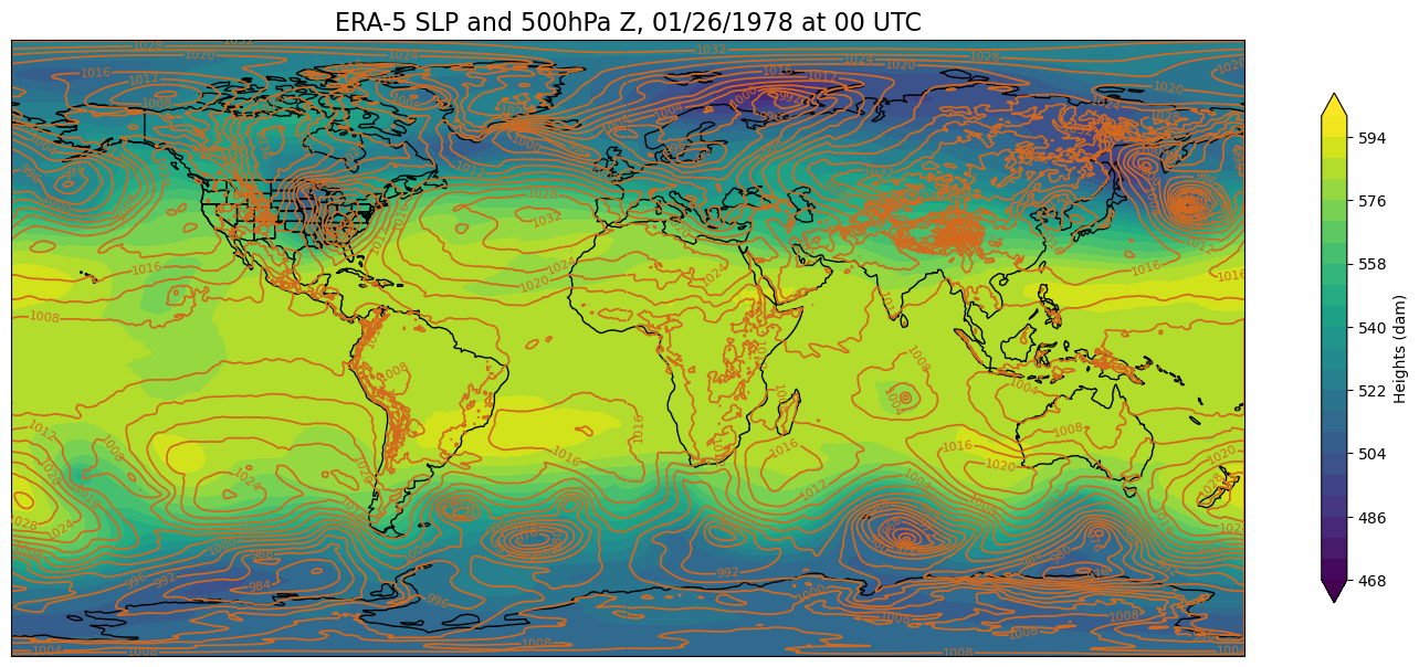
First, create a function that will create a global map using the Plate Carree projection. This is the projection that is used for visualizations on NOAA’s Science on a Sphere, such as the one we have here in ETEC!
def make_global_map(i, z):

    res = '110m'
    fig = plt.figure(figsize=(18,12))
    ax = plt.subplot(1,1,1,projection=ccrs.PlateCarree())
    ax.set_global()
    ax.add_feature(cfeature.COASTLINE.with_scale(res))
    ax.add_feature(cfeature.STATES.with_scale(res))

    # Add the title
    valTime = pd.to_datetime(SLP.time[i].values).strftime("%m/%d/%Y at %H UTC")
    tl1 = str("ERA-5 SLP and " + str(pLevel) + "hPa Z, " + valTime)
    plt.title(tl1,fontsize=16)

    # Height (Z) contour fills

    CF = ax.contourf(lons,lats,z,levels=zLevels,cmap=plt.get_cmap('viridis'), extend='both')
    cbar = fig.colorbar(CF,shrink=0.5)
    cbar.set_label(r'Heights (dam)', size='medium')

    # SLP contour lines
    CL = ax.contour(lons,lats,SLP.isel(time=i),slpLevels,linewidths=1.25,colors='chocolate')
    ax.clabel(CL, inline_spacing=0.2, fontsize=8, fmt='%.0f');
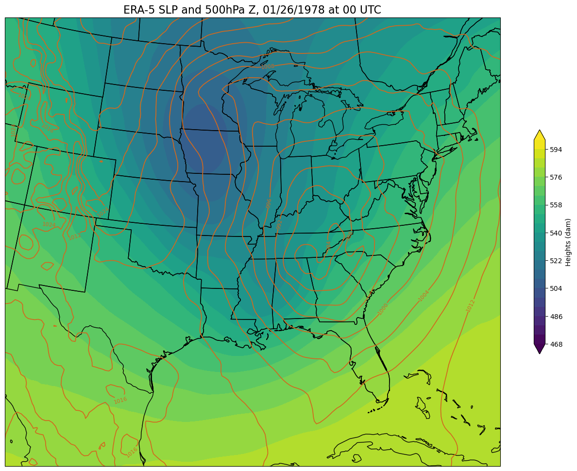
Now, create a regional map, focusing on our weather event of interest. First, set some values relevant to the regional map projection and extent.
lonW = -110.0
lonE = -70.0
latS = 20.0
latN = 50.0
cLon = (lonW + lonE) / 2.
cLat = (latS + latN) / 2.
proj_map = ccrs.LambertConformal(central_longitude=cLon, central_latitude=cLat)
proj_data = ccrs.PlateCarree() # Our data is lat-lon; thus its native projection is Plate Carree.
res = '50m'
constrainLon = 3.3
def make_regional_map(i, z):

    fig = plt.figure(figsize=(18, 12))
    ax = plt.subplot(1,1,1,projection=proj_map)
    ax.set_extent ([lonW + constrainLon,lonE - constrainLon,latS,latN])
    ax.add_feature(cfeature.COASTLINE.with_scale(res))
    ax.add_feature(cfeature.STATES.with_scale(res))

    # Add the title
    valTime = pd.to_datetime(SLP.time[i].values).strftime("%m/%d/%Y at %H UTC")
    tl1 = str("ERA-5 SLP and " + str(pLevel) + "hPa Z, " + valTime)
    plt.title(tl1,fontsize=16)

    # Height (Z) contour fills

    CF = ax.contourf(lons,lats,z,levels=zLevels,cmap=plt.get_cmap('viridis'), extend='both', transform=proj_data)
    cbar = fig.colorbar(CF,shrink=0.5)
    cbar.set_label(r'Heights (dam)', size='medium')

    # SLP contour lines
    CL = ax.contour(lons,lats,SLP.isel(time=i),slpLevels,linewidths=1.25,colors='chocolate', transform=proj_data)
    ax.clabel(CL, inline_spacing=0.2, fontsize=8, fmt='%.0f');
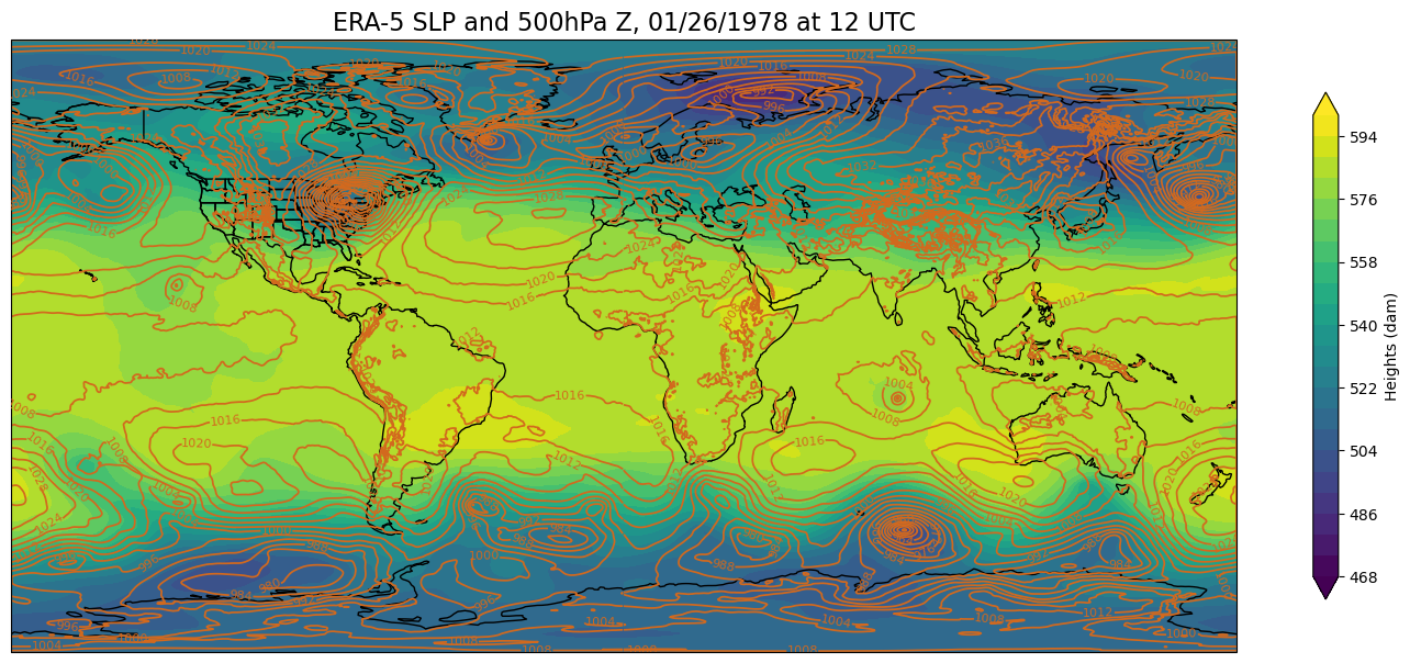
Create a for loop and loop through the times. In this loop, we will also pass in the geopotential grid, and convert its units from geopotential to decameters.
inc = 12 # change to 1 when you are ready
for time in range(0, 24, inc):
z = mpcalc.geopotential_to_height(Z.isel(time=time)).metpy.convert_units('dam')
make_global_map(time, z)
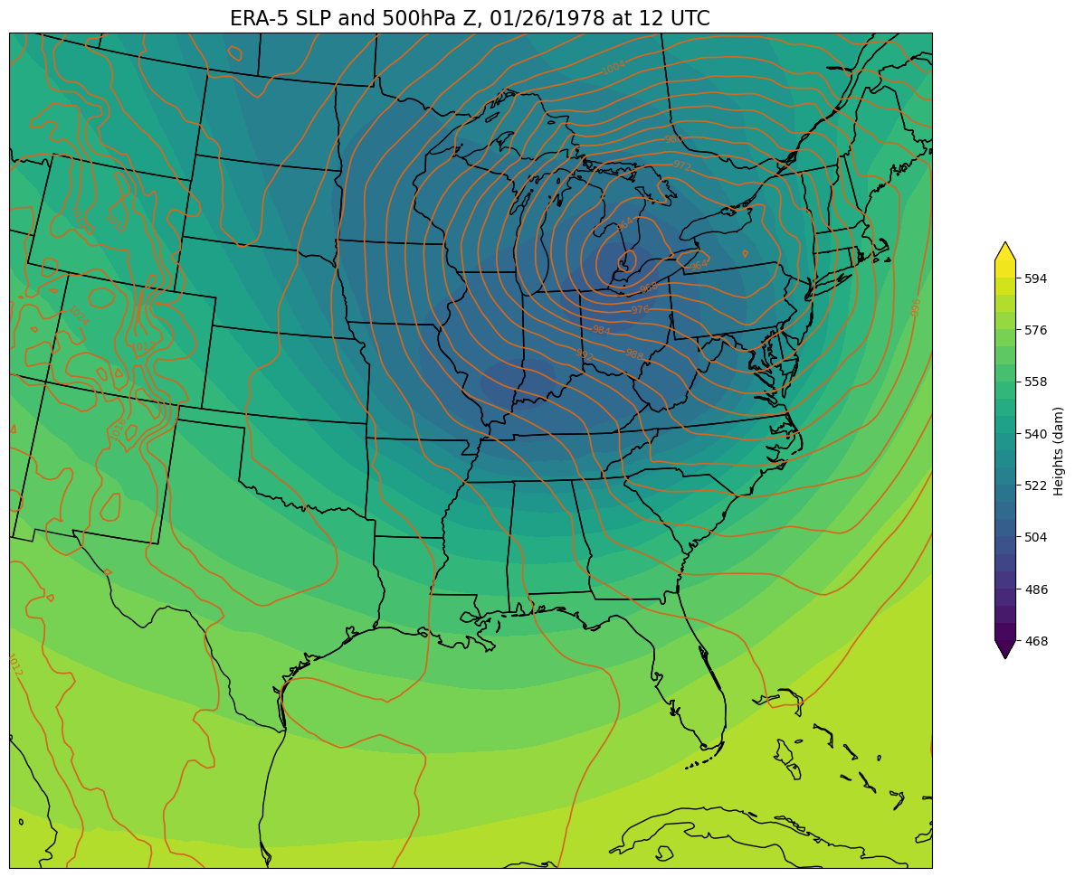
make_regional_map(time,z) # This will take some time, be patient!
print(time)
0
12
Things to try
Once you have run through this notebook, make a copy of it and choose another weather event. The ERA-5 now extends all the way back to 1950!!
Next, create some different visualizations, using the many variables in the ERA-5. For example:
850 hPa heights and temperature
300 hPa heights and isotachs
Snow depth
Accumulated precipitation
Sea surface temperature
“The sky’s the limit!” (or, “There is an endless sea of possibilities!”)
Ultimately, you and your team members will create 4 different 24-hour time loops for the weather event you have chosen.
What’s next?
In the next notebook, we will create a similar set of graphics, but save them to disk in a format amenable for loading on our Science on a Sphere!