Xarray 3: Datasets and Plotting
Contents
Xarray 3: Datasets and Plotting
Overview
The Xarray
DatasetOpen and select a variable from the ERA-5 dataset
Convert geopotential to height
Create a contour plot
Imports
import xarray as xr
import numpy as np
from metpy.units import units
import metpy.calc as mpcalc
import cartopy.crs as ccrs
import cartopy.feature as cfeature
import matplotlib.pyplot as plt
ERROR 1: PROJ: proj_create_from_database: Open of /knight/anaconda_aug22/envs/aug22_env/share/proj failed
Work with an Xarray Dataset
An Xarray Dataset consists of one or more DataArrays. Let’s open the same NetCDF file as in the first Xarray notebook, but as a Dataset.
ds = xr.open_dataset('/spare11/atm533/data/2012103000_z500_era5.nc')
Let’s see what this Dataset looks like.
ds
<xarray.Dataset>
Dimensions:    (longitude: 1440, latitude: 721, time: 1)
Coordinates:
  * longitude  (longitude) float32 0.0 0.25 0.5 0.75 ... 359.0 359.2 359.5 359.8
  * latitude   (latitude) float32 90.0 89.75 89.5 89.25 ... -89.5 -89.75 -90.0
  * time       (time) datetime64[ns] 2012-10-30
Data variables:
    z          (time, latitude, longitude) float32 ...
Attributes:
    Conventions:  CF-1.6
history: 2020-09-29 00:40:14 GMT by grib_to_netcdf-2.16.0: /opt/ecmw...It’s represented somewhat similarly to a DataArray, but now we have support for multiple data variables. In this case,
There is just one data variable: z (Geopotential)
The coordinate variables are longitude, latitude, and time
The data variable has three dimensions (time x latitude x longitude).
Although time is a dimension, there is only one time value on that coordinate.
The Dataset itself has attributes. The attributes of the coordinate and data variables are separately accessible.
Select a data variable from the Dataset.
Z = ds['z'] # Similar to selecting a Series in Pandas
We can programmatically retrieve various attributes of the data variable that we browsed interactively above.
Z
<xarray.DataArray 'z' (time: 1, latitude: 721, longitude: 1440)>
[1038240 values with dtype=float32]
Coordinates:
  * longitude  (longitude) float32 0.0 0.25 0.5 0.75 ... 359.0 359.2 359.5 359.8
  * latitude   (latitude) float32 90.0 89.75 89.5 89.25 ... -89.5 -89.75 -90.0
  * time       (time) datetime64[ns] 2012-10-30
Attributes:
    units:          m**2 s**-2
    long_name:      Geopotential
standard_name: geopotentialZ.shape
(1, 721, 1440)
Z.dims
('time', 'latitude', 'longitude')
We see that Z is a 3-dimensional DataArray, with time as the first dimension.
Z.units
'm**2 s**-2'
Convert geopotential to height
Print out the representation of our data variable. We can see it’s a DataArray.
print (Z) # Text-based, as opposed to HTML-prettified output
<xarray.DataArray 'z' (time: 1, latitude: 721, longitude: 1440)>
[1038240 values with dtype=float32]
Coordinates:
  * longitude  (longitude) float32 0.0 0.25 0.5 0.75 ... 359.0 359.2 359.5 359.8
  * latitude   (latitude) float32 90.0 89.75 89.5 89.25 ... -89.5 -89.75 -90.0
  * time       (time) datetime64[ns] 2012-10-30
Attributes:
    units:          m**2 s**-2
    long_name:      Geopotential
    standard_name:  geopotential
The units are already part of the data variable. We can use MetPy’s units and calc libraries to convert geopotential to height. We’ll assign a new object to the output of the function.
HGHT = mpcalc.geopotential_to_height(Z)
Print out its representation. Note that the array values have changed, and there is a unit attached to the DataArray.
print (HGHT)
<xarray.DataArray (time: 1, latitude: 721, longitude: 1440)>
<Quantity([[[5212.1777 5212.1777 5212.1777 ... 5212.1777 5212.1777 5212.1777]
  [5209.8657 5209.8657 5209.8823 ... 5209.8154 5209.832  5209.832 ]
  [5207.554  5207.5874 5207.604  ... 5207.4873 5207.504  5207.5376]
  ...
  [4974.5474 4974.5474 4974.564  ... 4974.497  4974.497  4974.514 ]
  [4970.8623 4970.8623 4970.8623 ... 4970.845  4970.845  4970.845 ]
  [4967.161  4967.161  4967.161  ... 4967.161  4967.161  4967.161 ]]], 'meter')>
Coordinates:
  * longitude  (longitude) float32 0.0 0.25 0.5 0.75 ... 359.0 359.2 359.5 359.8
  * latitude   (latitude) float32 90.0 89.75 89.5 89.25 ... -89.5 -89.75 -90.0
  * time       (time) datetime64[ns] 2012-10-30
Now we can make a map with contours of 500 hPa height!
Create a contour plot of gridded data
We will use Cartopy and Matplotlib to plot our 500 hPa height contours. Matplotlib has two contour methods:
Line contours: ax.contour
Filled contours: ax.contourf
We will draw contour lines in meters, with a contour interval of 60 m.
As we’ve done before, let’s first define some variables relevant to Cartopy.
cLon = -80
cLat = 35
lonW = -100
lonE = -60
latS = 20
latN = 50
proj_map = ccrs.LambertConformal(central_longitude=cLon, central_latitude=cLat)
proj_data = ccrs.PlateCarree() # Our data is lat-lon; thus its native projection is Plate Carree.
res = '50m'
Now define the range of our contour values and a contour interval. 60 m is standard for 500 hPa.
minVal = 4680
maxVal = 6060
cint = 60
cintervals = np.arange(minVal, maxVal, cint)
cintervals
array([4680, 4740, 4800, 4860, 4920, 4980, 5040, 5100, 5160, 5220, 5280,
       5340, 5400, 5460, 5520, 5580, 5640, 5700, 5760, 5820, 5880, 5940,
       6000])
Matplotlib’s contour methods require three arrays to be passed to them … x- and y- arrays (longitude and latitude in our case), and a 2-d array (corresponding to x- and y-) of our data variable. So we need to extract the latitude and longitude coordinate variables from our DataArray. We’ll also extract the third coordinate value, time.
lats = ds.latitude
lons = ds.longitude
times = ds.time
We’re set to make our map. After creating our figure, setting the bounds of our map domain, and adding cartographic features, we will plot the contours. We’ll assign the output of the contour method to an object, which will then be used to label the contour lines.
fig = plt.figure(figsize=(18,12))
ax = plt.subplot(1,1,1,projection=proj_map)
ax.set_extent ([lonW,lonE,latS,latN])
ax.add_feature(cfeature.COASTLINE.with_scale(res))
ax.add_feature(cfeature.STATES.with_scale(res))
CL = ax.contour(lons,lats,HGHT,cintervals,transform=proj_data,linewidths=1.25,colors='green')
ax.clabel(CL, inline_spacing=0.2, fontsize=11, fmt='%.0f');
---------------------------------------------------------------------------
TypeError                                 Traceback (most recent call last)
Input In [15], in <cell line: 6>()
      4 ax.add_feature(cfeature.COASTLINE.with_scale(res))
      5 ax.add_feature(cfeature.STATES.with_scale(res))
----> 6 CL = ax.contour(lons,lats,HGHT,cintervals,transform=proj_data,linewidths=1.25,colors='green')
      7 ax.clabel(CL, inline_spacing=0.2, fontsize=11, fmt='%.0f')

File /knight/anaconda_aug22/envs/aug22_env/lib/python3.10/site-packages/cartopy/mpl/geoaxes.py:318, in _add_transform.<locals>.wrapper(self, *args, **kwargs)
    313     raise ValueError(f'Invalid transform: Spherical {func.__name__} '
    314                      'is not supported - consider using '
    315                      'PlateCarree/RotatedPole.')
    317 kwargs['transform'] = transform
--> 318 return func(self, *args, **kwargs)

File /knight/anaconda_aug22/envs/aug22_env/lib/python3.10/site-packages/cartopy/mpl/geoaxes.py:362, in _add_transform_first.<locals>.wrapper(self, *args, **kwargs)
    360     # Use the new points as the input arguments
    361     args = (x, y, z) + args[3:]
--> 362 return func(self, *args, **kwargs)

File /knight/anaconda_aug22/envs/aug22_env/lib/python3.10/site-packages/cartopy/mpl/geoaxes.py:1614, in GeoAxes.contour(self, *args, **kwargs)
   1592 @_add_transform
   1593 @_add_transform_first
   1594 def contour(self, *args, **kwargs):
   1595     """
   1596     Add the "transform" keyword to :func:`~matplotlib.pyplot.contour`.
   1597
   (...)
   1612
   1613     """
-> 1614     result = super().contour(*args, **kwargs)
   1616     # We need to compute the dataLim correctly for contours.
   1617     bboxes = [col.get_datalim(self.transData)
   1618               for col in result.collections
   1619               if col.get_paths()]

File /knight/anaconda_aug22/envs/aug22_env/lib/python3.10/site-packages/matplotlib/__init__.py:1414, in _preprocess_data.<locals>.inner(ax, data, *args, **kwargs)
   1411 @functools.wraps(func)
   1412 def inner(ax, *args, data=None, **kwargs):
   1413     if data is None:
-> 1414         return func(ax, *map(sanitize_sequence, args), **kwargs)
   1416     bound = new_sig.bind(ax, *args, **kwargs)
   1417     auto_label = (bound.arguments.get(label_namer)
   1418                   or bound.kwargs.get(label_namer))

File /knight/anaconda_aug22/envs/aug22_env/lib/python3.10/site-packages/matplotlib/axes/_axes.py:6303, in Axes.contour(self, *args, **kwargs)
   6294 """
   6295 Plot contour lines.
   6296
   (...)
   6300 %(contour_doc)s
   6301 """
   6302 kwargs['filled'] = False
-> 6303 contours = mcontour.QuadContourSet(self, *args, **kwargs)
   6304 self._request_autoscale_view()
   6305 return contours

File /knight/anaconda_aug22/envs/aug22_env/lib/python3.10/site-packages/matplotlib/contour.py:812, in ContourSet.__init__(self, ax, levels, filled, linewidths, linestyles, hatches, alpha, origin, extent, cmap, colors, norm, vmin, vmax, extend, antialiased, nchunk, locator, transform, *args, **kwargs)
    808     self.origin = mpl.rcParams['image.origin']
    810 self._transform = transform
--> 812 kwargs = self._process_args(*args, **kwargs)
    813 self._process_levels()
    815 self._extend_min = self.extend in ['min', 'both']

File /knight/anaconda_aug22/envs/aug22_env/lib/python3.10/site-packages/matplotlib/contour.py:1446, in QuadContourSet._process_args(self, corner_mask, *args, **kwargs)
   1443     corner_mask = mpl.rcParams['contour.corner_mask']
   1444 self._corner_mask = corner_mask
-> 1446 x, y, z = self._contour_args(args, kwargs)
   1448 _mask = ma.getmask(z)
   1449 if _mask is ma.nomask or not _mask.any():

File /knight/anaconda_aug22/envs/aug22_env/lib/python3.10/site-packages/matplotlib/contour.py:1485, in QuadContourSet._contour_args(self, args, kwargs)
   1483     args = args[1:]
   1484 elif Nargs <= 4:
-> 1485     x, y, z = self._check_xyz(args[:3], kwargs)
   1486     args = args[3:]
   1487 else:

File /knight/anaconda_aug22/envs/aug22_env/lib/python3.10/site-packages/matplotlib/contour.py:1513, in QuadContourSet._check_xyz(self, args, kwargs)
   1510 z = ma.asarray(args[2], dtype=np.float64)
   1512 if z.ndim != 2:
-> 1513     raise TypeError(f"Input z must be 2D, not {z.ndim}D")
   1514 if z.shape[0] < 2 or z.shape[1] < 2:
   1515     raise TypeError(f"Input z must be at least a (2, 2) shaped array, "
   1516                     f"but has shape {z.shape}")

TypeError: Input z must be 2D, not 3D
Didn't work! The end of the traceback reads:
TypeError: Input z must be 2D, not 3D
In other words, our geopotential height array is not two dimensional in x and y ... recall that it also has *time* as its first dimension! Even though there is only one time value in this dimension, we need to eliminate this dimension from Z.
We’ll learn other ways to abstract out dimensions other than x and y (remember, there could be additional dimensions in our Datasets or DataArrays, such as vertical levels or ensemble members) in later notebooks, but for now, we can simply select the first (and only) element from the time dimension.
HGHT = HGHT[0,:,:] # Select the first element of the leading (time) dimension, and all lons and lats.
HGHT
<xarray.DataArray (latitude: 721, longitude: 1440)>
<Quantity([[5212.1777 5212.1777 5212.1777 ... 5212.1777 5212.1777 5212.1777]
 [5209.8657 5209.8657 5209.8823 ... 5209.8154 5209.832  5209.832 ]
 [5207.554  5207.5874 5207.604  ... 5207.4873 5207.504  5207.5376]
 ...
 [4974.5474 4974.5474 4974.564  ... 4974.497  4974.497  4974.514 ]
 [4970.8623 4970.8623 4970.8623 ... 4970.845  4970.845  4970.845 ]
 [4967.161  4967.161  4967.161  ... 4967.161  4967.161  4967.161 ]], 'meter')>
Coordinates:
  * longitude  (longitude) float32 0.0 0.25 0.5 0.75 ... 359.0 359.2 359.5 359.8
  * latitude   (latitude) float32 90.0 89.75 89.5 89.25 ... -89.5 -89.75 -90.0
time datetime64[ns] 2012-10-30Now try again.
fig = plt.figure(figsize=(18,12))
ax = plt.subplot(1,1,1,projection=proj_map)
ax.set_extent ([lonW,lonE,latS,latN])
ax.add_feature(cfeature.COASTLINE.with_scale(res))
ax.add_feature(cfeature.STATES.with_scale(res))
CL = ax.contour(lons,lats,HGHT,cintervals,transform=proj_data,linewidths=1.25,colors='green')
ax.clabel(CL, inline_spacing=0.2, fontsize=11, fmt='%.0f');
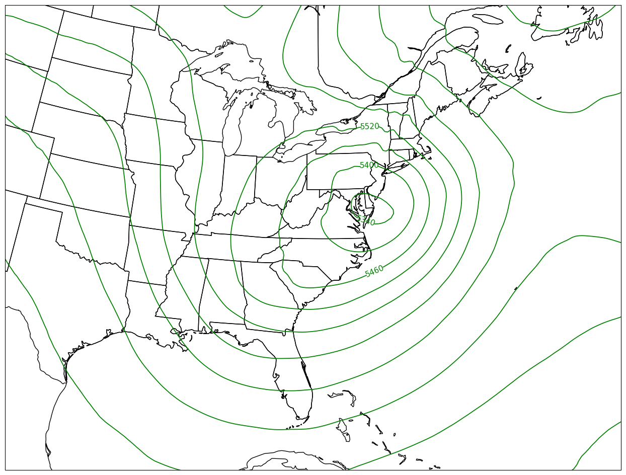
There we have it! There are definitely some things we can improve about this plot (such as the lack of an informative title, and the fact that our contour labels seem not to be appearing on every contour line), but we’ll get to that soon!
Summary
An Xarray
Datasetconsists of one or moreDataArrays.MetPy can perform unit-aware calculations and conversions on Xarray objects.
Since Xarray
DataArrays often have more than x- and y- dimensions, care must be taken to reduce dimensionality for the purposes of Matplotlib functions such ascontourandcontourf.
What’s Next?
In the next notebook, we’ll work with multiple Datasets.