Plotting archived HRRR data: 1km reflectivity
Contents

Plotting archived HRRR data: 1km reflectivity
Overview
Access archived HRRR data hosted on AWS in Zarr format
Visualize one of the variables (1km reflectivity) at an analysis time
Use one of MetPy’s customized color tables
Create and visualize a reflectivity time loop of all forecast hours in an archived HRRR run
Prerequisites
Concepts |
Importance |
Notes |
|---|---|---|
Zarr, Dask, S3 storage |
2mT notebook |
Necessary |
Time to learn: 30 minutes
Imports
import xarray as xr
import s3fs
import metpy
import numpy as np
import matplotlib.pyplot as plt
import cartopy.crs as ccrs
import cartopy.feature as cfeature
from metpy.plots import colortables
import pandas as pd
ERROR 1: PROJ: proj_create_from_database: Open of /knight/anaconda_aug22/envs/aug22_env/share/proj failed
Access the Zarr-formatted data on AWS
As in the 2m temperature notebook, create objects pointing to the HRRR S3 bucket and object of interest.
To access Zarr-formatted data stored in an S3 bucket, we follow a 3-step process:
Create URL(s) pointing to the bucket and object(s) that contain the data we want
Create map(s) to the object(s) with the s3fs library’s
S3MapmethodPass the map(s) to Xarray’s
open_datasetoropen_mfdatasetmethods, and specifyzarras the format, via theengineargument.
Create the URLs
date = '20221014'
hour = '00'
var = 'REFD'
level = '1000m_above_ground'
url1 = 's3://hrrrzarr/sfc/' + date + '/' + date + '_' + hour + 'z_anl.zarr/' + level + '/' + var + '/' + level
url2 = 's3://hrrrzarr/sfc/' + date + '/' + date + '_' + hour + 'z_anl.zarr/' + level + '/' + var
print(url1)
print(url2)
s3://hrrrzarr/sfc/20221014/20221014_00z_anl.zarr/1000m_above_ground/REFD/1000m_above_ground
s3://hrrrzarr/sfc/20221014/20221014_00z_anl.zarr/1000m_above_ground/REFD
Create the S3 maps from the S3 object store.
fs = s3fs.S3FileSystem(anon=True)
file1 = s3fs.S3Map(url1, s3=fs)
file2 = s3fs.S3Map(url2, s3=fs)
Use Xarray’s open_mfdataset to create a Dataset from these two S3 objects.
ds = xr.open_mfdataset([file1,file2], engine='zarr')
Examine the dataset.
ds
<xarray.Dataset>
Dimensions:                  (projection_y_coordinate: 1059,
                              projection_x_coordinate: 1799)
Coordinates:
  * projection_x_coordinate  (projection_x_coordinate) float64 -2.698e+06 ......
  * projection_y_coordinate  (projection_y_coordinate) float64 -1.587e+06 ......
Data variables:
    REFD                     (projection_y_coordinate, projection_x_coordinate) float16 dask.array<chunksize=(150, 150), meta=np.ndarray>
    forecast_period          timedelta64[ns] ...
    forecast_reference_time  datetime64[ns] ...
    height                   float64 ...
    pressure                 float64 ...
time datetime64[ns] ...Remind ourselves of the HRRR’s projection info:
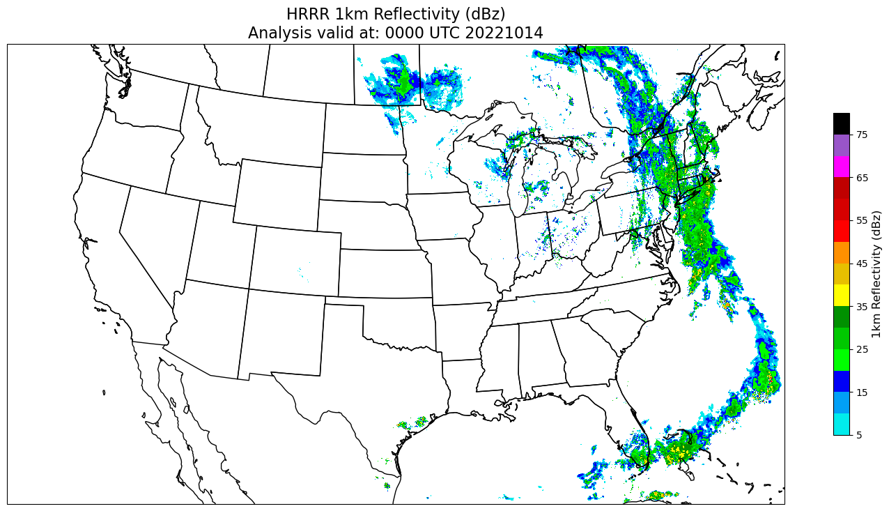
Visualize 1km Reflectivity at an analysis time
norm, cmap = colortables.get_with_range('NWSReflectivity', 5,80)
Examine the cmap object
cmap

Set the color map so values under the specified range are shaded in white
cmap.set_under('w')
cmap
Plot the map
We’ll define the plot extent to nicely encompass the HRRR’s spatial domain.
latN = 50.4
latS = 24.25
lonW = -123.8
lonE = -71.2
res = '50m'
fig = plt.figure(figsize=(18,12))
ax = plt.subplot(1,1,1,projection=projData)
ax.set_extent ([lonW,lonE,latS,latN],crs=ccrs.PlateCarree())
ax.add_feature(cfeature.COASTLINE.with_scale(res))
ax.add_feature(cfeature.STATES.with_scale(res))
# Add the title
tl1 = str('HRRR 1km Reflectivity (dBz)')
tl2 = str('Analysis valid at: '+ hour + '00 UTC ' + date )
plt.title(tl1+'\n'+tl2,fontsize=16)
CM = ax.pcolormesh(x, y, scalar, norm=norm, cmap=cmap)
# Make a colorbar for the color mesh.
cbar = fig.colorbar(CM,shrink=0.5)
cbar.set_label(r'1km Reflectivity (dBz)', size='large')
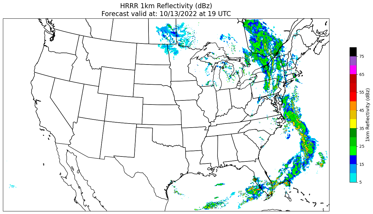
Now, create a loop of forecast radar reflectivity for a specific date and time in the archive.
The bucket/object are very similar; it’s fcst (forecast) instead of anl (analysis), though!
date = '20221013'
hour = '18'
var = 'REFD'
level = '1000m_above_ground'
url1 = 's3://hrrrzarr/sfc/' + date + '/' + date + '_' + hour + 'z_fcst.zarr/' + level + '/' + var + '/' + level
url2 = 's3://hrrrzarr/sfc/' + date + '/' + date + '_' + hour + 'z_fcst.zarr/' + level + '/' + var
print(url1)
print(url2)
s3://hrrrzarr/sfc/20221013/20221013_18z_fcst.zarr/1000m_above_ground/REFD/1000m_above_ground
s3://hrrrzarr/sfc/20221013/20221013_18z_fcst.zarr/1000m_above_ground/REFD
fs = s3fs.S3FileSystem(anon=True)
file1 = s3fs.S3Map(url1, s3=fs)
file2 = s3fs.S3Map(url2, s3=fs)
ds = xr.open_mfdataset([file1,file2], engine='zarr')
ds
<xarray.Dataset>
Dimensions: (time: 48, projection_y_coordinate: 1059,
projection_x_coordinate: 1799)
Coordinates:
  * projection_x_coordinate  (projection_x_coordinate) float64 -2.698e+06 ......
  * projection_y_coordinate  (projection_y_coordinate) float64 -1.587e+06 ......
* time (time) datetime64[ns] 2022-10-13T19:00:00 ... 20...
Data variables:
REFD (time, projection_y_coordinate, projection_x_coordinate) float16 dask.array<chunksize=(48, 150, 150), meta=np.ndarray>
forecast_period (time) timedelta64[ns] dask.array<chunksize=(48,), meta=np.ndarray>
forecast_reference_time datetime64[ns] ...The Dataset is very similar to the analysis; it just has a time dimension too! What times do we have available?
times = ds.time
times
<xarray.DataArray 'time' (time: 48)>
array(['2022-10-13T19:00:00.000000000', '2022-10-13T20:00:00.000000000',
       '2022-10-13T21:00:00.000000000', '2022-10-13T22:00:00.000000000',
       '2022-10-13T23:00:00.000000000', '2022-10-14T00:00:00.000000000',
       '2022-10-14T01:00:00.000000000', '2022-10-14T02:00:00.000000000',
       '2022-10-14T03:00:00.000000000', '2022-10-14T04:00:00.000000000',
       '2022-10-14T05:00:00.000000000', '2022-10-14T06:00:00.000000000',
       '2022-10-14T07:00:00.000000000', '2022-10-14T08:00:00.000000000',
       '2022-10-14T09:00:00.000000000', '2022-10-14T10:00:00.000000000',
       '2022-10-14T11:00:00.000000000', '2022-10-14T12:00:00.000000000',
       '2022-10-14T13:00:00.000000000', '2022-10-14T14:00:00.000000000',
       '2022-10-14T15:00:00.000000000', '2022-10-14T16:00:00.000000000',
       '2022-10-14T17:00:00.000000000', '2022-10-14T18:00:00.000000000',
       '2022-10-14T19:00:00.000000000', '2022-10-14T20:00:00.000000000',
       '2022-10-14T21:00:00.000000000', '2022-10-14T22:00:00.000000000',
       '2022-10-14T23:00:00.000000000', '2022-10-15T00:00:00.000000000',
       '2022-10-15T01:00:00.000000000', '2022-10-15T02:00:00.000000000',
       '2022-10-15T03:00:00.000000000', '2022-10-15T04:00:00.000000000',
       '2022-10-15T05:00:00.000000000', '2022-10-15T06:00:00.000000000',
       '2022-10-15T07:00:00.000000000', '2022-10-15T08:00:00.000000000',
       '2022-10-15T09:00:00.000000000', '2022-10-15T10:00:00.000000000',
       '2022-10-15T11:00:00.000000000', '2022-10-15T12:00:00.000000000',
       '2022-10-15T13:00:00.000000000', '2022-10-15T14:00:00.000000000',
       '2022-10-15T15:00:00.000000000', '2022-10-15T16:00:00.000000000',
       '2022-10-15T17:00:00.000000000', '2022-10-15T18:00:00.000000000'],
      dtype='datetime64[ns]')
Coordinates:
* time (time) datetime64[ns] 2022-10-13T19:00:00 ... 2022-10-15T18:00:00
Attributes:
long_name: timedef make_regional_map(i, z):
latN = 50.4
latS = 24.25
lonW = -123.8
lonE = -71.2
res = '50m'
fig = plt.figure(figsize=(18,12))
ax = plt.subplot(1,1,1,projection=projData)
ax.set_extent ([lonW,lonE,latS,latN],crs=ccrs.PlateCarree())
ax.add_feature(cfeature.COASTLINE.with_scale(res))
ax.add_feature(cfeature.STATES.with_scale(res))
# Add the title
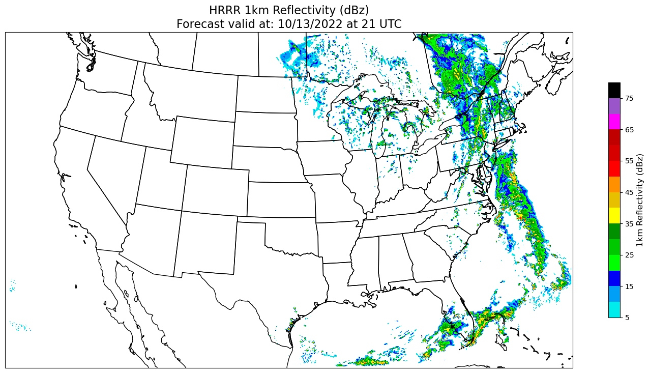
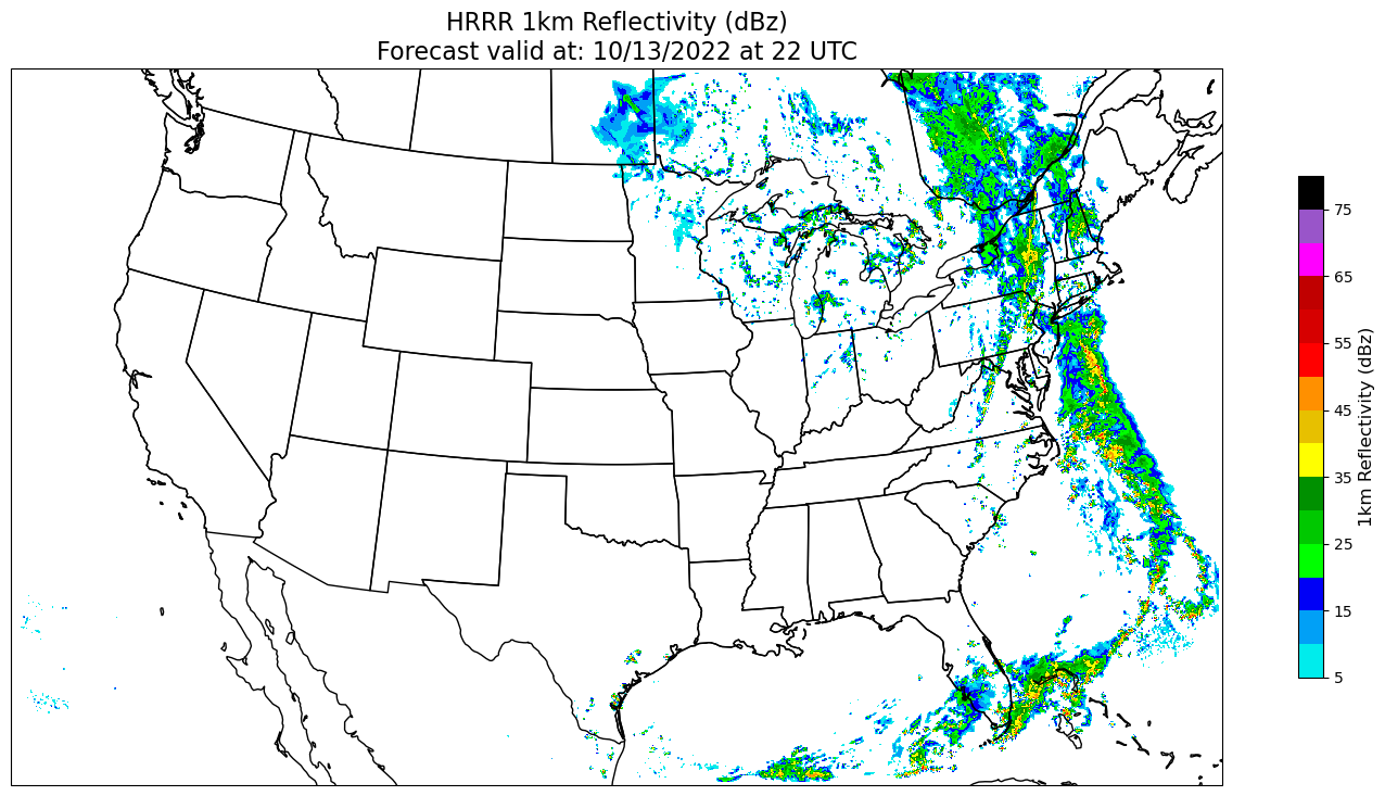
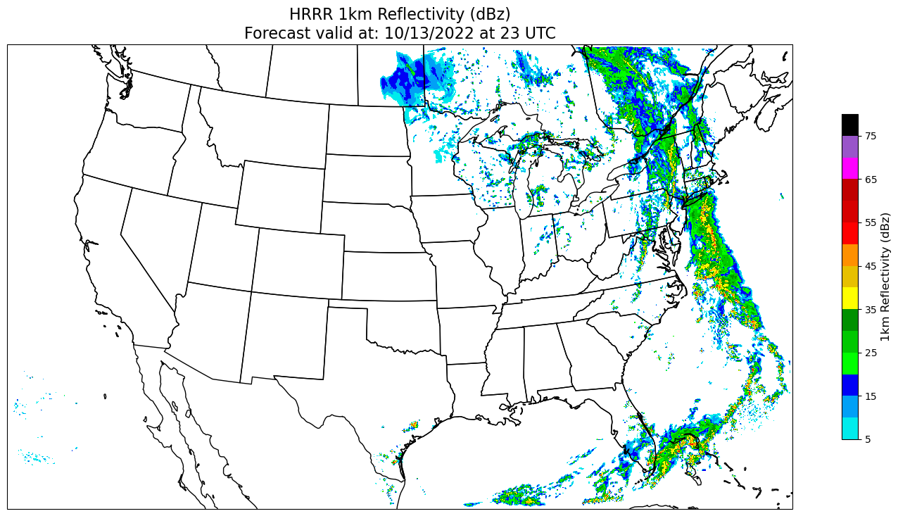
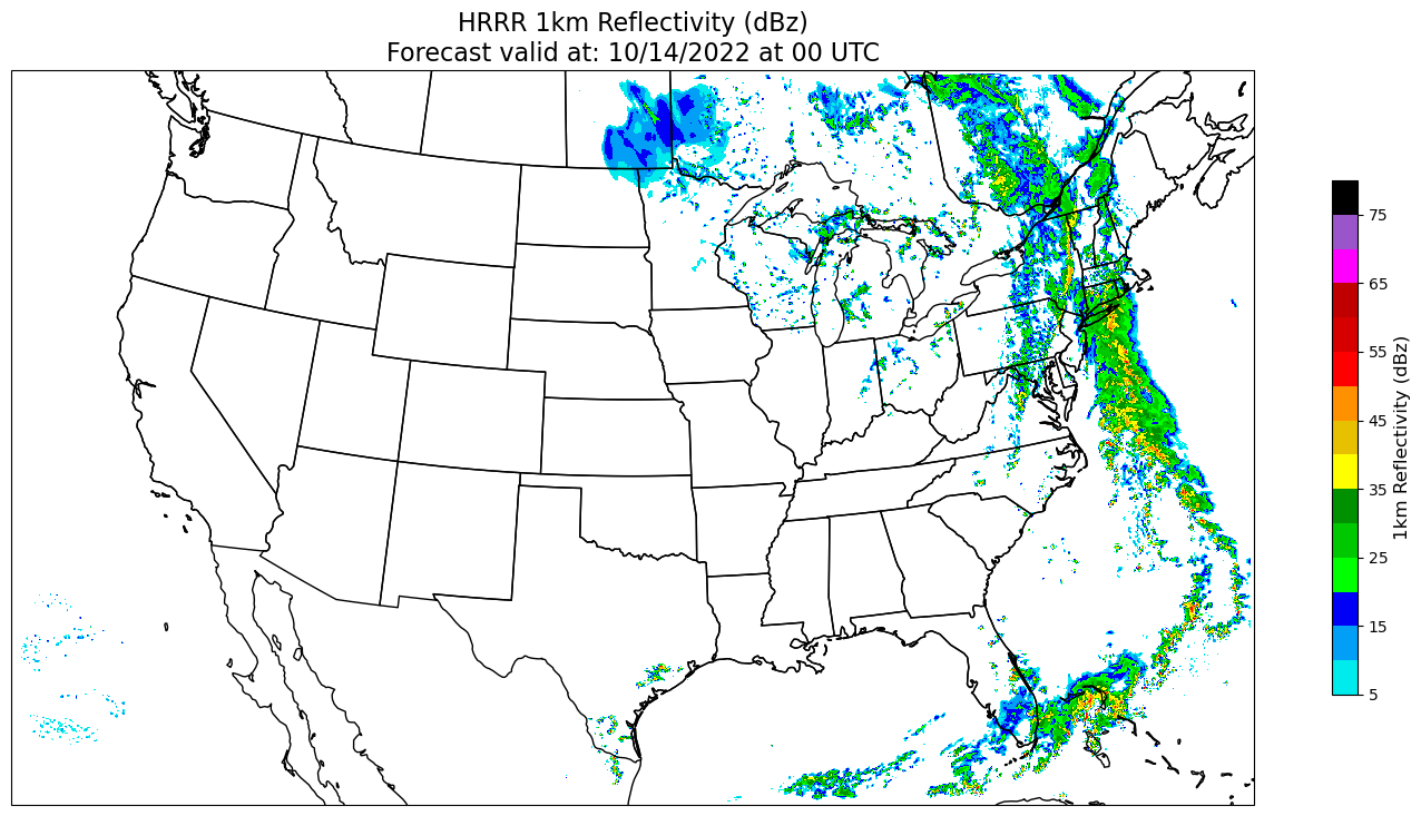
validTime = pd.to_datetime(z.time[i].values).strftime("%m/%d/%Y at %H UTC")
tl1 = str('HRRR 1km Reflectivity (dBz)')
tl2 = str('Forecast valid at: '+ validTime )
ax.set_title(tl1+'\n'+tl2,fontsize=16)
CM = ax.pcolormesh(z.projection_x_coordinate, z.projection_y_coordinate, z.isel(time=i), norm=norm, cmap=cmap)
# Make a colorbar for the color mesh.
cbar = fig.colorbar(CM,shrink=0.5)
cbar.set_label(r'1km Reflectivity (dBz)', size='large')
plt.show()
In the interest of time (pun intended), let’s just make a six-hour forecast loop. Revise as you desire!
parameter = 'REFD'
hrStart = 0
hrStop = 6
hrInc = 1
for i in range (hrStart, hrStop, hrInc):
    make_regional_map(i, ds[parameter])

Summary
With a minimum of changes, we can adapt our initial 2-meter temperature notebook to different HRRR variables, such as 1 km reflectivity.
Matplotlib’s
ax.pcolormeshfunction is ideal for plotting raster fields, such as radar reflectivity.Metpy’s
colortablesprovide several meteorologically-relevant color tables, which can be easily incorporated and modified in matplotlib.
Things to try
Save your maps to disk, instead of (or in addition to) within your notebook.
Create a map whose domain covers a smaller region … e.g. the Albany region, or another area of interest to you. If the region is small enough, consider adding MetPy’s county line outlines.
Create a near-realtime HRRR forecast loop. The most recent HRRR tends to appear on the AWS hrrrzarr bucket with an approximate 90-120 minute lag. Think about how you might dynamically determine the most recently available time, no matter when you run the notebook.
Besides the single-level parameters, located in the sfc folder of the hrrrzarr bucket, explore the ones on isobaric surfaces, in the prs folder (these are analysis times only, no forecasts).