Intro to Xarray
Contents
Intro to Xarray
Outline
Introduction to Xarray
Anatomy of a DataArray
Imports
import xarray as xr
While Pandas is great for many purposes, extending its inherently 2-d data representation to a multidimensional dataset, such as 4-dimensional (time, vertical level, longitude (x) and latitude (y)) gridded NWP/Climate model output, is unwise.
Gridded data is typically written in a non-ASCII (i.e., not human-readable) format. The two most widely-used formats are GRIB and NetCDF. These binary formats take up less storage space than text.
The Xarray package is ideally-suited for gridded data, in particular NetCDF. It builds and extends on the multi-dimensional data structure in NumPy. We will see that some of the same methods we’ve used for Pandas have analogues in Xarray.
As a a general introduction to Xarray, below is part of a section from the Xarray Tutorial that was presented at the SciPy 2020 conference:
(Start of SciPy 2020 Xarray Tutorial snippet)
Multi-dimensional (a.k.a. N-dimensional, ND) arrays (sometimes called “tensors”) are an essential part of computational science. They are encountered in a wide range of fields, including physics, astronomy, geoscience, bioinformatics, engineering, finance, and deep learning. In Python, NumPy provides the fundamental data structure and API for working with raw ND arrays. However, real-world datasets are usually more than just raw numbers; they have labels which encode information about how the array values map to locations in space, time, etc.
Here is an example of how we might structure a dataset for a weather forecast:
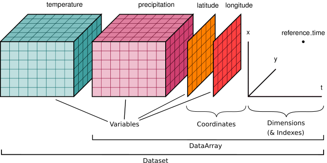
You’ll notice multiple data variables (temperature, precipitation), coordinate variables (latitude, longitude), and dimensions (x, y, t). We’ll cover how these fit into Xarray’s data structures below.
Xarray doesn’t just keep track of labels on arrays – it uses them to provide a powerful and concise interface, with methods that look a lot like Pandas. For example:
Apply operations over dimensions by name:
x.sum('time').Select values by label (or logical location) instead of integer location:
x.loc['2014-01-01']orx.sel(time='2014-01-01').Mathematical operations (e.g.,
x - y) vectorize across multiple dimensions (array broadcasting) based on dimension names, not shape.Easily use the split-apply-combine paradigm with groupby:
x.groupby('time.dayofyear').mean().Database-like alignment based on coordinate labels that smoothly handles missing values:
x, y = xr.align(x, y, join='outer').Keep track of arbitrary metadata in the form of a Python dictionary:
x.attrs.
The N-dimensional nature of xarray’s data structures makes it suitable for
dealing with multi-dimensional scientific data, and its use of dimension names
instead of axis labels (dim='time' instead of axis=0 or axis='columns') makes such arrays much
more manageable than the raw numpy ndarray: with xarray, you don’t need to keep
track of the order of an array’s dimensions or insert dummy dimensions of size 1
to align arrays (e.g., using np.newaxis).
The immediate payoff of using xarray is that you’ll write less code. The long-term payoff is that you’ll understand what you were thinking when you come back to look at it weeks or months later.
(End of SciPy 2020 Xarray Tutorial snippet)
Core XArray objects: the Dataset and the DataArray
As did Pandas with its Series and DataFrame core data structures, Xarray also has two “workhorses”: the DataArray and the Dataset. Just as a Pandas DataFrame consists of multiple Series, an Xarray Dataset is made up of one or more DataArray objects. Let’s first look at a couple of Datasets, that are Xarray’s representation of two of our in-house archive of Climate Forecast System Reanalysis (CFSR) gridded data files.
# Similar to a Pandas DataFrame, we get a nice (and even more interactive) HTML representation of the object.
year = 1993
ds_slp = xr.open_dataset(f'/cfsr/data/{year}/pmsl.1993.0p5.anl.nc')
ds_g = xr.open_dataset(f'/cfsr/data/{year}/g.1993.0p5.anl.nc')
ds_slp
<xarray.Dataset>
Dimensions:  (time: 1460, lat: 361, lon: 720)
Coordinates:
  * time     (time) datetime64[ns] 1993-01-01 ... 1993-12-31T18:00:00
  * lat      (lat) float32 -90.0 -89.5 -89.0 -88.5 -88.0 ... 88.5 89.0 89.5 90.0
  * lon      (lon) float32 -180.0 -179.5 -179.0 -178.5 ... 178.5 179.0 179.5
Data variables:
    pmsl     (time, lat, lon) float32 ...
Attributes:
    description:    pmsl as a single level variable
    year:           1993
    source:         http://nomads.ncdc.noaa.gov/data.php?name=access#CFSR-data
    references:     Saha, et. al., (2010)
    created_by:     User: kgriffin
creation_date: Wed Apr 4 05:59:11 UTC 2012The ds_slp Dataset has the following properties:
It has three named dimensions, in order: time, lat(itude), and lon(gitude).
It has three coordinate variables, which (in this case, but not always) correspond to the dimensions.
It contains one named data variable: ‘pmsl’. The data variable can be read in as a Data Array.
It has attributes which are the data variable’s metadata.
Its coordinate variables may have their own metadata as well.
Exercise:
Next, examine the ds_g Dataset.
# Write your code here
ds_g
<xarray.Dataset>
Dimensions: (time: 1460, lat: 361, lon: 720, lev: 32)
Coordinates:
* time (time) datetime64[ns] 1993-01-01 ... 1993-12-31T18:00:00
* lat (lat) float32 -90.0 -89.5 -89.0 -88.5 -88.0 ... 88.5 89.0 89.5 90.0
* lon (lon) float32 -180.0 -179.5 -179.0 -178.5 ... 178.5 179.0 179.5
* lev (lev) float32 1e+03 975.0 950.0 925.0 900.0 ... 50.0 30.0 20.0 10.0
Data variables:
g (time, lev, lat, lon) float32 ...
Attributes:
description: g 1000-10 hPa
year: 1993
source: http://nomads.ncdc.noaa.gov/data.php?name=access#CFSR-data
references: Saha, et. al., (2010)
created_by: User: kgriffin
creation_date: Wed Apr 4 05:58:31 UTC 2012How do the properties for the ds_g Dataset compare and contrast to the ds_slp one?
DataArrays
When we analyze and display information in a gridded Xarray Dataset, we are actually working with one or more DataArrays within one or more Datasets. In the CFSR sea-level pressure dataset, there exists one gridded field, pmsl. Let’s read it in as an Xarray DataArray object. You will see that we access it in a similar manner to how we accessed a column, aka Series, in a Pandas Dataframe.
slp = ds_slp['pmsl']
slp
<xarray.DataArray 'pmsl' (time: 1460, lat: 361, lon: 720)>
[379483200 values with dtype=float32]
Coordinates:
* time (time) datetime64[ns] 1993-01-01 ... 1993-12-31T18:00:00
* lat (lat) float32 -90.0 -89.5 -89.0 -88.5 -88.0 ... 88.5 89.0 89.5 90.0
* lon (lon) float32 -180.0 -179.5 -179.0 -178.5 ... 178.5 179.0 179.5
Attributes:
level_type: single level variable
units: Pa
long_name: pressure reduced mean sea levelSimilar to the ds_slp Dataset which contains it, this DataArray has the following properties:
It is a named data variable: ‘pmsl’
It has three named dimensions, in order: time, lat(itude), and lon(gitude).
It has three coordinate variables, which (in this case, but not always) correspond to the dimensions.
It has attributes which are the data variable’s metadata.
Its coordinate variables may have their own metadata as well.
Let’s examine each of these five properties.
1. The data variable, pmsl in this case, is represented by the DataArray object itself. We can query various properties of it, with methods similar to Pandas.
# Akin to column and row indices in Pandas:
slp.indexes
Indexes:
time DatetimeIndex(['1993-01-01 00:00:00', '1993-01-01 06:00:00',
'1993-01-01 12:00:00', '1993-01-01 18:00:00',
'1993-01-02 00:00:00', '1993-01-02 06:00:00',
'1993-01-02 12:00:00', '1993-01-02 18:00:00',
'1993-01-03 00:00:00', '1993-01-03 06:00:00',
...
'1993-12-29 12:00:00', '1993-12-29 18:00:00',
'1993-12-30 00:00:00', '1993-12-30 06:00:00',
'1993-12-30 12:00:00', '1993-12-30 18:00:00',
'1993-12-31 00:00:00', '1993-12-31 06:00:00',
'1993-12-31 12:00:00', '1993-12-31 18:00:00'],
dtype='datetime64[ns]', name='time', length=1460, freq=None)
lat Index([-90.0, -89.5, -89.0, -88.5, -88.0, -87.5, -87.0, -86.5, -86.0, -85.5,
...
85.5, 86.0, 86.5, 87.0, 87.5, 88.0, 88.5, 89.0, 89.5, 90.0],
dtype='float32', name='lat', length=361)
lon Index([-180.0, -179.5, -179.0, -178.5, -178.0, -177.5, -177.0, -176.5, -176.0,
-175.5,
...
175.0, 175.5, 176.0, 176.5, 177.0, 177.5, 178.0, 178.5, 179.0,
179.5],
dtype='float32', name='lon', length=720)
slp.mean()
<xarray.DataArray 'pmsl' ()> array(100982.1, dtype=float32)
slp.max()
<xarray.DataArray 'pmsl' ()> array(106766.875)
slp.min()
<xarray.DataArray 'pmsl' ()> array(91299.5)
This invocation will return the lat, lon, and time of the minimum (or maximum) value in the DataArray (source: https://stackoverflow.com/questions/40179593/how-to-get-the-coordinates-of-the-maximum-in-xarray)
slp.where(slp==slp.min(), drop=True).coords
Coordinates:
* time (time) datetime64[ns] 1993-06-12T06:00:00
* lat (lat) float32 -63.0
* lon (lon) float32 2.5
We can use loc to select via dimension values, but note that order of indices must follow dimension order.
slp.loc['1993-03-14-18:00:00',42.5,-74.0]
<xarray.DataArray 'pmsl' ()>
array(99651.12, dtype=float32)
Coordinates:
time datetime64[ns] 1993-03-14T18:00:00
lat float32 42.5
lon float32 -74.0
Attributes:
level_type: single level variable
units: Pa
long_name: pressure reduced mean sea levelWe can alternatively, (and preferably!) use Xarray’s sel indexing technique, where we specify the names of the dimension and the values we are selecting … can be in any order … and does not need to include all dimensions. In the cell below, we get the SLP values for this particular point for every time in the dataset.
slp.sel(lon = -74.0, lat = 42.5)
<xarray.DataArray 'pmsl' (time: 1460)>
array([101087.47 , 101234.26 , 101707.9 , ..., 102255.695, 102277.64 ,
102122.16 ], dtype=float32)
Coordinates:
* time (time) datetime64[ns] 1993-01-01 ... 1993-12-31T18:00:00
lat float32 42.5
lon float32 -74.0
Attributes:
level_type: single level variable
units: Pa
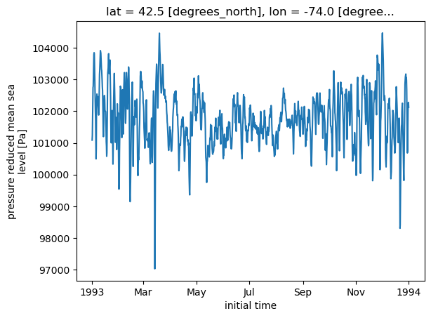
long_name: pressure reduced mean sea levelts = slp.sel(lon = -74.0, lat = 42.5)
ts.plot()
[<matplotlib.lines.Line2D at 0x14df565c3250>]
2. Dimension names
In Xarray, dimensions can be thought of as extensions of Pandas` 2-d row/column indices (aka axes). We can assign names, or labels, to Pandas indexes; in Xarray, these labeled axes are a necessary (and excellent) feature.
slp.dims
('time', 'lat', 'lon')
3. Coordinates
Coordinate variables in Xarray are 1-dimensional arrays that correspond to the Data variable’s dimensions.
In this case, slp has dimension coordinates of longitude, latitude, and time; each of these dimension coordinates consist of an array of values, plus metadata.
slp.coords
Coordinates:
* time (time) datetime64[ns] 1993-01-01 ... 1993-12-31T18:00:00
* lat (lat) float32 -90.0 -89.5 -89.0 -88.5 -88.0 ... 88.5 89.0 89.5 90.0
* lon (lon) float32 -180.0 -179.5 -179.0 -178.5 ... 178.5 179.0 179.5
We can assign an object to each coordinate dimension.
lons = slp.lon
lats = slp.lat
time = slp.time
time
<xarray.DataArray 'time' (time: 1460)>
array(['1993-01-01T00:00:00.000000000', '1993-01-01T06:00:00.000000000',
       '1993-01-01T12:00:00.000000000', ..., '1993-12-31T06:00:00.000000000',
       '1993-12-31T12:00:00.000000000', '1993-12-31T18:00:00.000000000'],
      dtype='datetime64[ns]')
Coordinates:
* time (time) datetime64[ns] 1993-01-01 ... 1993-12-31T18:00:00
Attributes:
actual_range: [1691808. 1700562.]
last_time: 1993-12-31 18:00:00
first_time: 1993-1-1 00:00:00
delta_t: 0000-00-00 06:00:00
long_name: initial time4. The data variables will typically have attributes (metadata) attached to them.
slp.attrs
{'level_type': 'single level variable',
'units': 'Pa',
'long_name': 'pressure reduced mean sea level'}
slp.units
'Pa'
5. The coordinate variables will likely have metadata as well.
time.attrs
{'actual_range': array([1691808., 1700562.]),
'last_time': '1993-12-31 18:00:00',
'first_time': '1993-1-1 00:00:00',
'delta_t': '0000-00-00 06:00:00',
'long_name': 'initial time'}
lats.attrs
{'actual_range': array([-90, 90], dtype=int32),
'delta_y': 0.5,
'coordinate_defines': 'center',
'mapping': 'cylindrical_equidistant_projection_grid',
'grid_resolution': '0.5_degrees',
'long_name': 'latitude',
'units': 'degrees_north'}
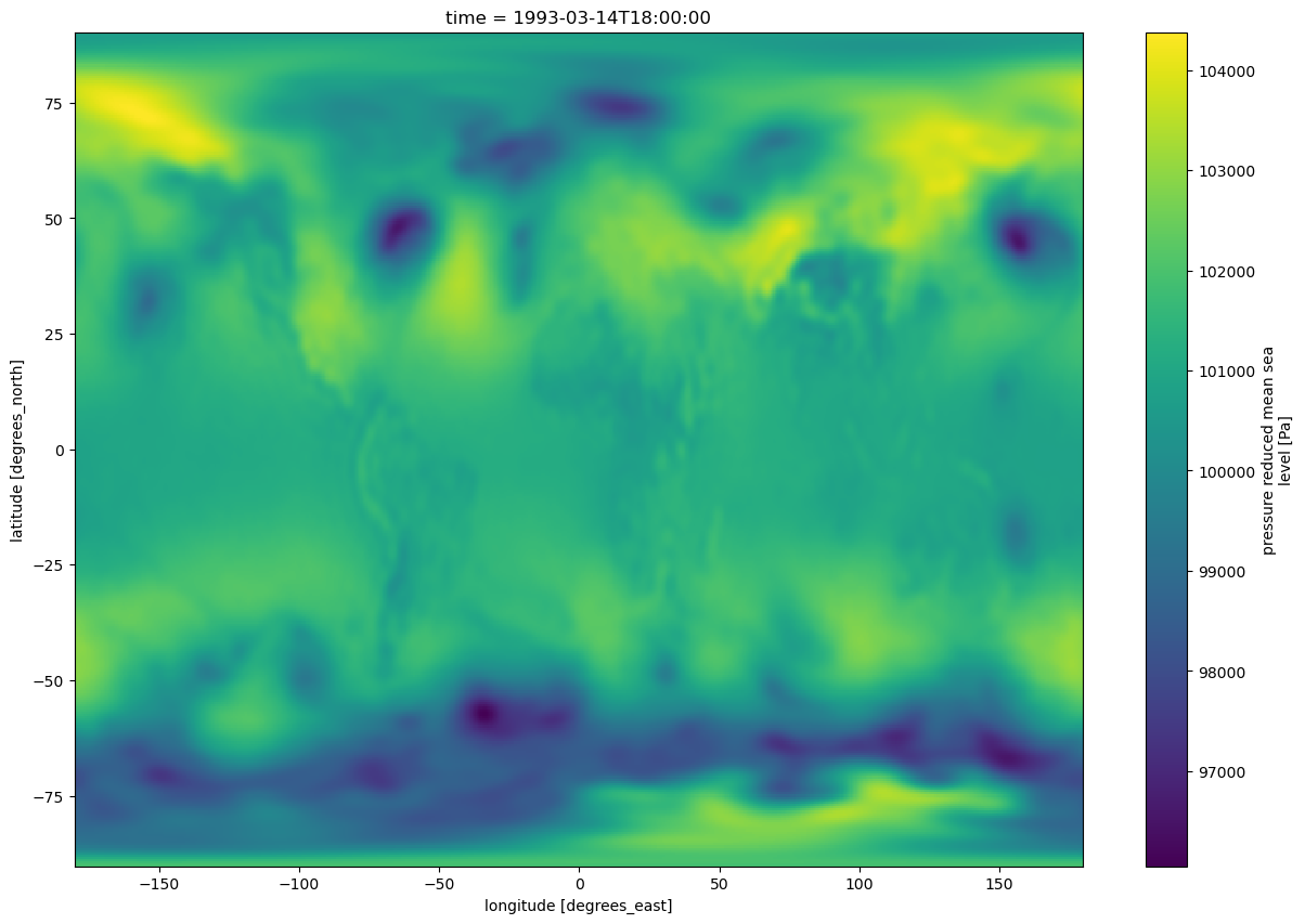
Just as with Pandas, Xarray has a built-in hook to Matplotlib so we can take a quick look at our data.
slp.sel(time='1993-03-14-18:00:00').plot(figsize=(15,10))
<matplotlib.collections.QuadMesh at 0x14df562a1190>
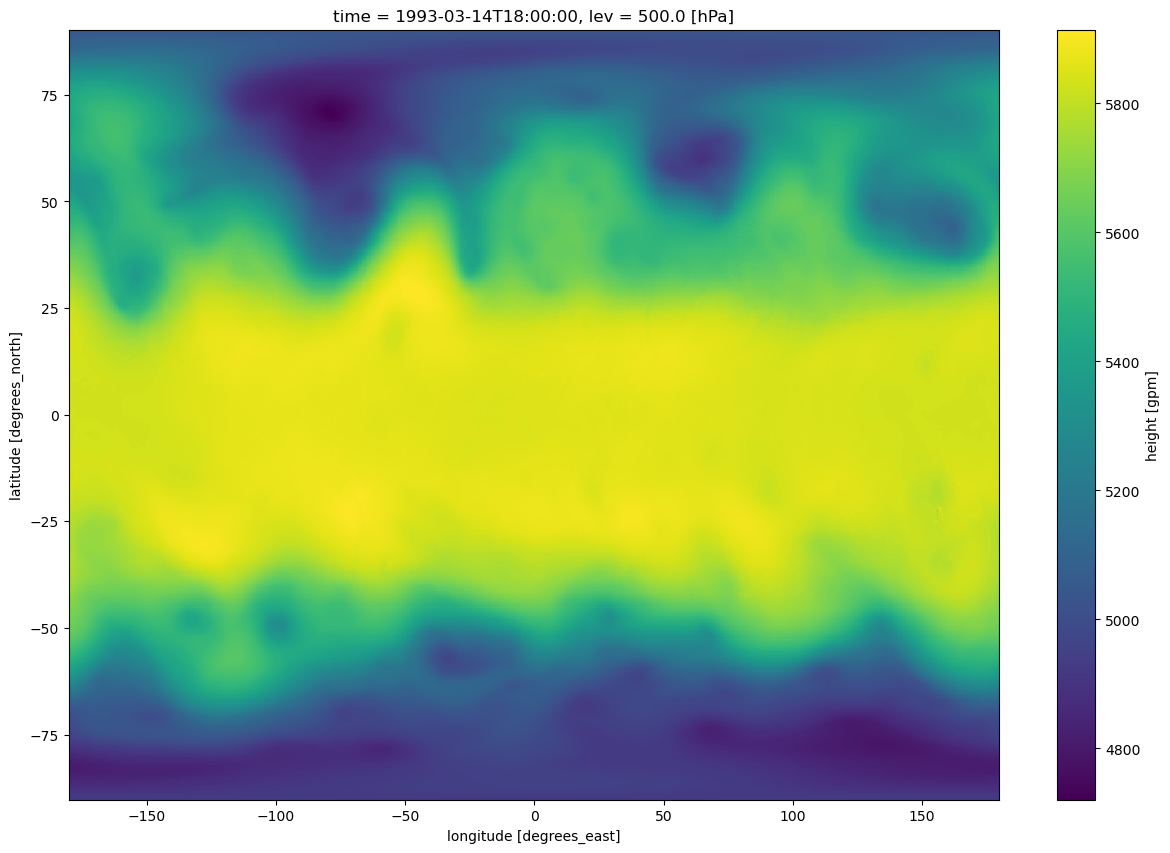
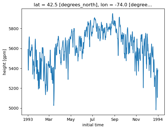
Exercise:
Write code cells that produce a quick plot of 500 hPa geopotential height over the entire domain and a time series of 500 hPa geopotential height at a specific latitude and longitude.
ds_g
<xarray.Dataset>
Dimensions:  (time: 1460, lat: 361, lon: 720, lev: 32)
Coordinates:
  * time     (time) datetime64[ns] 1993-01-01 ... 1993-12-31T18:00:00
  * lat      (lat) float32 -90.0 -89.5 -89.0 -88.5 -88.0 ... 88.5 89.0 89.5 90.0
  * lon      (lon) float32 -180.0 -179.5 -179.0 -178.5 ... 178.5 179.0 179.5
  * lev      (lev) float32 1e+03 975.0 950.0 925.0 900.0 ... 50.0 30.0 20.0 10.0
Data variables:
    g        (time, lev, lat, lon) float32 ...
Attributes:
    description:    g 1000-10 hPa
    year:           1993
    source:         http://nomads.ncdc.noaa.gov/data.php?name=access#CFSR-data
    references:     Saha, et. al., (2010)
    created_by:     User: kgriffin
creation_date: Wed Apr 4 05:58:31 UTC 2012z = ds_g['g']
z
<xarray.DataArray 'g' (time: 1460, lev: 32, lat: 361, lon: 720)>
[12143462400 values with dtype=float32]
Coordinates:
  * time     (time) datetime64[ns] 1993-01-01 ... 1993-12-31T18:00:00
  * lat      (lat) float32 -90.0 -89.5 -89.0 -88.5 -88.0 ... 88.5 89.0 89.5 90.0
  * lon      (lon) float32 -180.0 -179.5 -179.0 -178.5 ... 178.5 179.0 179.5
* lev (lev) float32 1e+03 975.0 950.0 925.0 900.0 ... 50.0 30.0 20.0 10.0
Attributes:
level_type: isobaric_level (hPa)
units: gpm
long_name: heightz500 = z.sel(lev=500)
z500
<xarray.DataArray 'g' (time: 1460, lat: 361, lon: 720)>
[379483200 values with dtype=float32]
Coordinates:
  * time     (time) datetime64[ns] 1993-01-01 ... 1993-12-31T18:00:00
  * lat      (lat) float32 -90.0 -89.5 -89.0 -88.5 -88.0 ... 88.5 89.0 89.5 90.0
  * lon      (lon) float32 -180.0 -179.5 -179.0 -178.5 ... 178.5 179.0 179.5
    lev      float32 500.0
Attributes:
    level_type:  isobaric_level (hPa)
    units:       gpm
long_name: heightts = z500.sel(lon = -74.0, lat = 42.5)
ts.plot()
[<matplotlib.lines.Line2D at 0x14df565ca490>]
z500.sel(time='1993-03-14-18:00:00').plot(figsize=(15,10))
<matplotlib.collections.QuadMesh at 0x14df4dc1a050>