Animating NEXRAD Level II Data
Contents
Animating NEXRAD Level II Data
Overview
Within this notebook, we will cover:
Exploring the “guts” of a NEXRAD radar file
Animating a sequence of AWS-served NEXRAD Level 2 Radar scans
Prerequisites
Concepts |
Importance |
Notes |
|---|---|---|
Required |
Projections and Features |
|
Required |
Basic plotting |
|
Py-ART Basics |
Required |
IO/Visualization |
Time to learn: 20 minutes
Imports
import pyart
import fsspec
from metpy.plots import USCOUNTIES, ctables
import matplotlib.pyplot as plt
import cartopy.crs as ccrs
import cartopy.feature as cfeature
import warnings
from datetime import datetime as dt
from datetime import timedelta

import matplotlib
matplotlib.rcParams['animation.html'] = 'html5'
from matplotlib.animation import ArtistAnimation

warnings.filterwarnings("ignore")
## You are using the Python ARM Radar Toolkit (Py-ART), an open source
## library for working with weather radar data. Py-ART is partly
## supported by the U.S. Department of Energy as part of the Atmospheric
## Radiation Measurement (ARM) Climate Research Facility, an Office of
## Science user facility.
##
## If you use this software to prepare a publication, please cite:
##
##     JJ Helmus and SM Collis, JORS 2016, doi: 10.5334/jors.119
Select the time and NEXRAD site
datTime = dt(2014,5,26,22)
year = dt.strftime(datTime,format="%Y")
month = dt.strftime(datTime,format="%m")
day = dt.strftime(datTime,format="%d")
hour = dt.strftime(datTime,format="%H")
timeStr = f'{year}{month}{day}{hour}'

site = 'KSJT'
Point to the NOAA NEXRAD Level 2 S3 Bucket on AWS
fs = fsspec.filesystem("s3", anon=True)
Depending on the year, the radar files will have different naming conventions.
pattern1 = f's3://noaa-nexrad-level2/{year}/{month}/{day}/{site}/{site}{year}{month}{day}_{hour}*V06'
pattern2 = f's3://noaa-nexrad-level2/{year}/{month}/{day}/{site}/{site}{year}{month}{day}_{hour}*V*.gz'
pattern3 = f's3://noaa-nexrad-level2/{year}/{month}/{day}/{site}/{site}{year}{month}{day}_{hour}*.gz'
Construct the URL pointing to the radar file directory and get a list of matching files.
Try each file pattern. Once the list of files is non-empty, we are all set.
files = sorted(fs.glob(pattern1))

if (len(files) == 0):
    files = sorted(fs.glob(pattern2))

if (len(files) == 0):
    files = sorted(fs.glob(pattern3))
If we still have an empty list, either there are no files available for that site/date, or the file name does not match any of the patterns above.
if (len(files) == 0):
    print ("There are no files found for this date and location. Either try a different date/site, \
or browse the NEXRAD2 archive to see if the file name uses a different pattern.")
else:
    print (files)
['noaa-nexrad-level2/2014/05/26/KSJT/KSJT20140526_220132_V06.gz', 'noaa-nexrad-level2/2014/05/26/KSJT/KSJT20140526_220504_V06.gz', 'noaa-nexrad-level2/2014/05/26/KSJT/KSJT20140526_220850_V06.gz', 'noaa-nexrad-level2/2014/05/26/KSJT/KSJT20140526_221222_V06.gz', 'noaa-nexrad-level2/2014/05/26/KSJT/KSJT20140526_221607_V06.gz', 'noaa-nexrad-level2/2014/05/26/KSJT/KSJT20140526_221954_V06.gz', 'noaa-nexrad-level2/2014/05/26/KSJT/KSJT20140526_222339_V06.gz', 'noaa-nexrad-level2/2014/05/26/KSJT/KSJT20140526_222724_V06.gz', 'noaa-nexrad-level2/2014/05/26/KSJT/KSJT20140526_223110_V06.gz', 'noaa-nexrad-level2/2014/05/26/KSJT/KSJT20140526_223455_V06.gz', 'noaa-nexrad-level2/2014/05/26/KSJT/KSJT20140526_223840_V06.gz', 'noaa-nexrad-level2/2014/05/26/KSJT/KSJT20140526_224225_V06.gz', 'noaa-nexrad-level2/2014/05/26/KSJT/KSJT20140526_224610_V06.gz', 'noaa-nexrad-level2/2014/05/26/KSJT/KSJT20140526_224956_V06.gz', 'noaa-nexrad-level2/2014/05/26/KSJT/KSJT20140526_225341_V06.gz', 'noaa-nexrad-level2/2014/05/26/KSJT/KSJT20140526_225740_V06.gz']
Read the Data into PyART
Read in the first radar file in the group and list the available fields.
radar = pyart.io.read_nexrad_archive(f's3://{files[0]}')
list(radar.fields)
['differential_phase',
 'reflectivity',
 'spectrum_width',
 'velocity',
 'cross_correlation_ratio',
 'differential_reflectivity']
The radar object has a lot of useful data … and metadata! One way to look at the attributes of any Python object is to use the vars function. It returns a Python dictionary; each dictionary key has an associated value … which might be a single value … a list of values … another dictionary … and so on.
radarDict = vars(radar)
radarDict
{'time': {'units': 'seconds since 2014-05-26T22:01:32Z',
  'standard_name': 'time',
  'long_name': 'time_in_seconds_since_volume_start',
  'calendar': 'gregorian',
  'comment': 'Coordinate variable for time. Time at the center of each ray, in fractional seconds since the global variable time_coverage_start',
  'data': array([  0.84 ,   0.865,   0.883, ..., 204.719, 204.754, 204.79 ])},
 'range': {'units': 'meters',
  'standard_name': 'projection_range_coordinate',
  'long_name': 'range_to_measurement_volume',
  'axis': 'radial_range_coordinate',
  'spacing_is_constant': 'true',
  'comment': 'Coordinate variable for range. Range to center of each bin.',
  'data': array([  2125.,   2375.,   2625., ..., 459375., 459625., 459875.],
        dtype=float32),
  'meters_to_center_of_first_gate': 2125.0,
  'meters_between_gates': 250.0},
 'fields': {'differential_phase': {'units': 'degrees',
   'standard_name': 'differential_phase_hv',
   'long_name': 'differential_phase_hv',
   'valid_max': 360.0,
   'valid_min': 0.0,
   'coordinates': 'elevation azimuth range',
   '_FillValue': -9999.0,
   'data': masked_array(
     data=[[24.32918357849121, 19.3928279876709, 16.572052001953125, ...,
            --, --, --],
           [8.10972785949707, 7.051937103271484, 5.288952827453613, ..., --,
            --, --],
           [68.75638580322266, 63.82003402709961, 58.17848205566406, ...,
            --, --, --],
           ...,
           [24.681779861450195, 33.14410400390625, 34.20189666748047, ...,
            --, --, --],
           [35.612281799316406, 40.54863739013672, 27.50255584716797, ...,
            --, --, --],
           [25.73957061767578, 41.95902633666992, 53.24212646484375, ...,
            --, --, --]],
     mask=[[False, False, False, ...,  True,  True,  True],
           [False, False, False, ...,  True,  True,  True],
           [False, False, False, ...,  True,  True,  True],
           ...,
           [False, False, False, ...,  True,  True,  True],
           [False, False, False, ...,  True,  True,  True],
           [False, False, False, ...,  True,  True,  True]],
     fill_value=1e+20,
     dtype=float32)},
  'reflectivity': {'units': 'dBZ',
   'standard_name': 'equivalent_reflectivity_factor',
   'long_name': 'Reflectivity',
   'valid_max': 94.5,
   'valid_min': -32.0,
   'coordinates': 'elevation azimuth range',
   '_FillValue': -9999.0,
   'data': masked_array(
     data=[[14.0, 16.0, 17.5, ..., --, --, --],
           [13.5, 13.5, 13.5, ..., --, --, --],
           [6.5, 7.0, 7.0, ..., --, --, --],
           ...,
           [-2.0, 13.0, 5.5, ..., --, --, --],
           [7.0, 2.0, 1.0, ..., --, --, --],
           [11.5, 9.5, -9.0, ..., --, --, --]],
     mask=[[False, False, False, ...,  True,  True,  True],
           [False, False, False, ...,  True,  True,  True],
           [False, False, False, ...,  True,  True,  True],
           ...,
           [False, False, False, ...,  True,  True,  True],
           [False, False, False, ...,  True,  True,  True],
           [False, False, False, ...,  True,  True,  True]],
     fill_value=1e+20,
     dtype=float32)},
  'spectrum_width': {'units': 'meters_per_second',
   'standard_name': 'doppler_spectrum_width',
   'long_name': 'Spectrum Width',
   'valid_max': 63.0,
   'valid_min': -63.5,
   'coordinates': 'elevation azimuth range',
   '_FillValue': -9999.0,
   'data': masked_array(
     data=[[--, --, --, ..., --, --, --],
           [--, --, --, ..., --, --, --],
           [--, --, --, ..., --, --, --],
           ...,
           [1.0, 1.0, 0.0, ..., --, --, --],
           [1.0, 0.0, 1.0, ..., --, --, --],
           [0.0, 1.0, 0.0, ..., --, --, --]],
     mask=[[ True,  True,  True, ...,  True,  True,  True],
           [ True,  True,  True, ...,  True,  True,  True],
           [ True,  True,  True, ...,  True,  True,  True],
           ...,
           [False, False, False, ...,  True,  True,  True],
           [False, False, False, ...,  True,  True,  True],
           [False, False, False, ...,  True,  True,  True]],
     fill_value=1e+20,
     dtype=float32)},
  'velocity': {'units': 'meters_per_second',
   'standard_name': 'radial_velocity_of_scatterers_away_from_instrument',
   'long_name': 'Mean doppler Velocity',
   'valid_max': 95.0,
   'valid_min': -95.0,
   'coordinates': 'elevation azimuth range',
   '_FillValue': -9999.0,
   'data': masked_array(
     data=[[--, --, --, ..., --, --, --],
           [--, --, --, ..., --, --, --],
           [--, --, --, ..., --, --, --],
           ...,
           [8.0, 7.0, 7.5, ..., --, --, --],
           [8.0, 8.0, 8.0, ..., --, --, --],
           [7.5, 7.0, 9.5, ..., --, --, --]],
     mask=[[ True,  True,  True, ...,  True,  True,  True],
           [ True,  True,  True, ...,  True,  True,  True],
           [ True,  True,  True, ...,  True,  True,  True],
           ...,
           [False, False, False, ...,  True,  True,  True],
           [False, False, False, ...,  True,  True,  True],
           [False, False, False, ...,  True,  True,  True]],
     fill_value=1e+20,
     dtype=float32)},
  'cross_correlation_ratio': {'units': 'ratio',
   'standard_name': 'cross_correlation_ratio_hv',
   'long_name': 'Cross correlation_ratio (RHOHV)',
   'valid_max': 1.0,
   'valid_min': 0.0,
   'coordinates': 'elevation azimuth range',
   '_FillValue': -9999.0,
   'data': masked_array(
     data=[[0.721666693687439, 0.7183333039283752, 0.7183333039283752, ...,
            --, --, --],
           [0.9283333420753479, 0.8883333206176758, 0.824999988079071, ...,
            --, --, --],
           [0.7350000143051147, 0.7850000262260437, 0.9049999713897705, ...,
            --, --, --],
           ...,
           [0.7916666865348816, 0.9883333444595337, 0.9950000047683716, ...,
            --, --, --],
           [0.9983333349227905, 0.9516666531562805, 0.9483333230018616, ...,
            --, --, --],
           [0.9950000047683716, 0.971666693687439, 0.2083333283662796, ...,
            --, --, --]],
     mask=[[False, False, False, ...,  True,  True,  True],
           [False, False, False, ...,  True,  True,  True],
           [False, False, False, ...,  True,  True,  True],
           ...,
           [False, False, False, ...,  True,  True,  True],
           [False, False, False, ...,  True,  True,  True],
           [False, False, False, ...,  True,  True,  True]],
     fill_value=1e+20,
     dtype=float32)},
  'differential_reflectivity': {'units': 'dB',
   'standard_name': 'log_differential_reflectivity_hv',
   'long_name': 'log_differential_reflectivity_hv',
   'valid_max': 7.9375,
   'valid_min': -7.875,
   'coordinates': 'elevation azimuth range',
   '_FillValue': -9999.0,
   'data': masked_array(
     data=[[5.25, 5.1875, 5.125, ..., --, --, --],
           [7.8125, 7.75, 7.5625, ..., --, --, --],
           [6.375, 7.9375, 7.9375, ..., --, --, --],
           ...,
           [7.9375, 7.9375, 7.9375, ..., --, --, --],
           [7.9375, 6.875, 7.9375, ..., --, --, --],
           [7.9375, 7.9375, 7.9375, ..., --, --, --]],
     mask=[[False, False, False, ...,  True,  True,  True],
           [False, False, False, ...,  True,  True,  True],
           [False, False, False, ...,  True,  True,  True],
           ...,
           [False, False, False, ...,  True,  True,  True],
           [False, False, False, ...,  True,  True,  True],
           [False, False, False, ...,  True,  True,  True]],
     fill_value=1e+20,
     dtype=float32)}},
 'metadata': {'Conventions': 'CF/Radial instrument_parameters',
  'version': '1.3',
  'title': '',
  'institution': '',
  'references': '',
  'source': '',
  'history': '',
  'comment': '',
  'instrument_name': 'KSJT',
  'original_container': 'NEXRAD Level II',
  'vcp_pattern': 212},
 'scan_type': 'ppi',
 'latitude': {'long_name': 'Latitude',
  'standard_name': 'Latitude',
  'units': 'degrees_north',
  'data': array([31.37111092])},
 'longitude': {'long_name': 'Longitude',
  'standard_name': 'Longitude',
  'units': 'degrees_east',
  'data': array([-100.49222565])},
 'altitude': {'long_name': 'Altitude',
  'standard_name': 'Altitude',
  'units': 'meters',
  'positive': 'up',
  'data': array([610.])},
 'altitude_agl': None,
 'sweep_number': {'units': 'count',
  'standard_name': 'sweep_number',
  'long_name': 'Sweep number',
  'data': array([ 0,  1,  2,  3,  4,  5,  6,  7,  8,  9, 10, 11], dtype=int32)},
 'sweep_mode': {'units': 'unitless',
  'standard_name': 'sweep_mode',
  'long_name': 'Sweep mode',
  'comment': 'Options are: "sector", "coplane", "rhi", "vertical_pointing", "idle", "azimuth_surveillance", "elevation_surveillance", "sunscan", "pointing", "manual_ppi", "manual_rhi"',
  'data': array([b'azimuth_surveillance', b'azimuth_surveillance',
         b'azimuth_surveillance', b'azimuth_surveillance',
         b'azimuth_surveillance', b'azimuth_surveillance',
         b'azimuth_surveillance', b'azimuth_surveillance',
         b'azimuth_surveillance', b'azimuth_surveillance',
         b'azimuth_surveillance', b'azimuth_surveillance'], dtype='|S20')},
 'fixed_angle': {'long_name': 'Target angle for sweep',
  'units': 'degrees',
  'standard_name': 'target_fixed_angle',
  'data': array([0.48339844, 0.48339844, 0.87890625, 0.87890625, 1.3183594 ,
         1.3183594 , 1.8017578 , 2.4169922 , 3.1201172 , 3.9990234 ,
         5.0976562 , 6.4160156 ], dtype=float32)},
 'sweep_start_ray_index': {'long_name': 'Index of first ray in sweep, 0-based',
  'units': 'count',
  'data': array([   0,  720, 1440, 2160, 2880, 3600, 4320, 4680, 5040, 5400, 5760,
         6120], dtype=int32)},
 'sweep_end_ray_index': {'long_name': 'Index of last ray in sweep, 0-based',
  'units': 'count',
  'data': array([ 719, 1439, 2159, 2879, 3599, 4319, 4679, 5039, 5399, 5759, 6119,
         6479], dtype=int32)},
 'target_scan_rate': None,
 'rays_are_indexed': None,
 'ray_angle_res': None,
 'azimuth': {'units': 'degrees',
  'standard_name': 'beam_azimuth_angle',
  'long_name': 'azimuth_angle_from_true_north',
  'axis': 'radial_azimuth_coordinate',
  'comment': 'Azimuth of antenna relative to true north',
  'data': array([119.25384521, 119.72900391, 120.17120361, ..., 334.50622559,
         335.50048828, 336.51123047])},
 'elevation': {'units': 'degrees',
  'standard_name': 'beam_elevation_angle',
  'long_name': 'elevation_angle_from_horizontal_plane',
  'axis': 'radial_elevation_coordinate',
  'comment': 'Elevation of antenna relative to the horizontal plane',
  'data': array([0.69488525, 0.6427002 , 0.6564331 , ..., 6.4160156 , 6.4160156 ,
         6.4160156 ], dtype=float32)},
 'scan_rate': None,
 'antenna_transition': None,
 'rotation': None,
 'tilt': None,
 'roll': None,
 'drift': None,
 'heading': None,
 'pitch': None,
 'georefs_applied': None,
 'instrument_parameters': {'unambiguous_range': {'units': 'meters',
   'comments': 'Unambiguous range',
   'meta_group': 'instrument_parameters',
   'long_name': 'Unambiguous range',
   'data': array([466000., 466000., 466000., ..., 117000., 117000., 117000.],
         dtype=float32)},
  'nyquist_velocity': {'units': 'meters_per_second',
   'comments': 'Unambiguous velocity',
   'meta_group': 'instrument_parameters',
   'long_name': 'Nyquist velocity',
   'data': array([ 8.35,  8.35,  8.35, ..., 33.26, 33.26, 33.26], dtype=float32)}},
 'radar_calibration': None,
 'ngates': 1832,
 'nrays': 6480,
 'nsweeps': 12,
 'projection': {'proj': 'pyart_aeqd', '_include_lon_0_lat_0': True},
 'rays_per_sweep': <pyart.lazydict.LazyLoadDict at 0x1543abd863d0>,
 'gate_x': <pyart.lazydict.LazyLoadDict at 0x1543abd86450>,
 'gate_y': <pyart.lazydict.LazyLoadDict at 0x1543abd86510>,
 'gate_z': <pyart.lazydict.LazyLoadDict at 0x1543abd86590>,
 'gate_longitude': <pyart.lazydict.LazyLoadDict at 0x1543abd86650>,
 'gate_latitude': <pyart.lazydict.LazyLoadDict at 0x1543abd86710>,
 'gate_altitude': <pyart.lazydict.LazyLoadDict at 0x1543abd867d0>}
We can get a list of all the individual keys in the dictionary:
radarDict.keys()
dict_keys(['time', 'range', 'fields', 'metadata', 'scan_type', 'latitude', 'longitude', 'altitude', 'altitude_agl', 'sweep_number', 'sweep_mode', 'fixed_angle', 'sweep_start_ray_index', 'sweep_end_ray_index', 'target_scan_rate', 'rays_are_indexed', 'ray_angle_res', 'azimuth', 'elevation', 'scan_rate', 'antenna_transition', 'rotation', 'tilt', 'roll', 'drift', 'heading', 'pitch', 'georefs_applied', 'instrument_parameters', 'radar_calibration', 'ngates', 'nrays', 'nsweeps', 'projection', 'rays_per_sweep', 'gate_x', 'gate_y', 'gate_z', 'gate_longitude', 'gate_latitude', 'gate_altitude'])
The first key is time. Let’s look at it:
radarDict['time']
{'units': 'seconds since 2014-05-26T22:01:32Z',
 'standard_name': 'time',
 'long_name': 'time_in_seconds_since_volume_start',
 'calendar': 'gregorian',
 'comment': 'Coordinate variable for time. Time at the center of each ray, in fractional seconds since the global variable time_coverage_start',
 'data': array([  0.84 ,   0.865,   0.883, ..., 204.719, 204.754, 204.79 ])}
It’s also a Python dictionary! It’s shorter than its parent’s … so we can see that there are six keys. Let’s look at the first one, units.
radarDict['time']['units']
'seconds since 2014-05-26T22:01:32Z'
It’s a string … and a useful one … as it provides a base time that we can use to infer timestamps for the start of each of the individual sweeps that make up the full volume scan of this particular radar file.
Let’s look at time’s data key:
radar.time['data'] # equivalent to: radarDict['time']['data']
array([ 0.84 , 0.865, 0.883, ..., 204.719, 204.754, 204.79 ])
radar dictionary can be accessed as an attribute in the radar object itself. How many elements are in this array?
len(radar.time['data'])
6480
Other keys include longitude and latitude. Let’s have a look at them:
radarDict['longitude'], radarDict['latitude']
({'long_name': 'Longitude',
  'standard_name': 'Longitude',
  'units': 'degrees_east',
  'data': array([-100.49222565])},
 {'long_name': 'Latitude',
  'standard_name': 'Latitude',
  'units': 'degrees_north',
  'data': array([31.37111092])})
These are also dictionaries! What do you think the data keys represent in both of them?
# %load /spare11/atm350/common/apr23/radarDict.py
radarDict['elevation']['data']
array([0.69488525, 0.6427002 , 0.6564331 , ..., 6.4160156 , 6.4160156 ,
       6.4160156 ], dtype=float32)
What is the length of the data array associated with elevation?
len(radarDict['elevation']['data'])
6480
radarDict['elevation']['data'][:30]
array([0.69488525, 0.6427002 , 0.6564331 , 0.6399536 , 0.6838989 ,
       0.67840576, 0.703125  , 0.6591797 , 0.65093994, 0.5932617 ,
       0.6097412 , 0.6152344 , 0.63720703, 0.6591797 , 0.6591797 ,
       0.6591797 , 0.6591797 , 0.6591797 , 0.6591797 , 0.6591797 ,
       0.6591797 , 0.6591797 , 0.6591797 , 0.6591797 , 0.6591797 ,
       0.6591797 , 0.6591797 , 0.6591797 , 0.6591797 , 0.6591797 ],
      dtype=float32)
Let’s see …
radarDict['sweep_start_ray_index']
{'long_name': 'Index of first ray in sweep, 0-based',
 'units': 'count',
 'data': array([   0,  720, 1440, 2160, 2880, 3600, 4320, 4680, 5040, 5400, 5760,
        6120], dtype=int32)}
radarDict['sweep_end_ray_index']
{'long_name': 'Index of last ray in sweep, 0-based',
 'units': 'count',
 'data': array([ 719, 1439, 2159, 2879, 3599, 4319, 4679, 5039, 5399, 5759, 6119,
        6479], dtype=int32)}
cLon, cLat = radar.longitude['data'], radar.latitude['data']
cLon, cLat
(array([-100.49222565]), array([31.37111092]))
Specify latitude and longitude bounds for the resulting maps, the resolution of the cartographic shapefiles, and the desired sweep level.
lonW = cLon - 2
lonE = cLon + 2
latS = cLat - 2
latN = cLat + 2
domain = lonW, lonE, latS, latN

res = '10m'
sweep = 0
Define a function that will determine at which ray a particular sweep begins; also define some strings for the figure title.
def nexRadSweepTimeElev (radar, sweep):

    sweepRayIndex = radar.sweep_start_ray_index['data'][sweep]

    baseTimeStr = radar.time['units'].split()[-1]
    baseTime = dt.strptime(baseTimeStr, "%Y-%m-%dT%H:%M:%SZ")

    timeSweep = baseTime + timedelta(seconds=radar.time['data'][sweepRayIndex])

    timeSweepStr = dt.strftime(timeSweep, format="%Y-%m-%d %H:%M:%S UTC")

    elevSweep = radar.fixed_angle['data'][sweep]
    elevSweepStr = f'{elevSweep:.1f}°'
    return timeSweepStr, elevSweepStr
radar.sweep_start_ray_index
{'long_name': 'Index of first ray in sweep, 0-based',
 'units': 'count',
 'data': array([   0,  720, 1440, 2160, 2880, 3600, 4320, 4680, 5040, 5400, 5760,
        6120], dtype=int32)}
radar.sweep_number
{'units': 'count',
 'standard_name': 'sweep_number',
 'long_name': 'Sweep number',
 'data': array([ 0,  1,  2,  3,  4,  5,  6,  7,  8,  9, 10, 11], dtype=int32)}
field = 'reflectivity'
shortName = 'REFL'
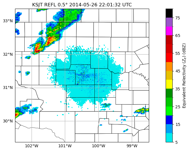
Create a single figure of reflectivity, zoomed into the area of interest.
# Creating color tables for reflectivity (every 5 dBZ starting with 5 dBZ):
ref_norm, ref_cmap = ctables.registry.get_with_steps('NWSReflectivity', 5, 5)
ref_cmap

# Call the function that creates the title string, among other things.
timeSweepStr, elevSweepStr = nexRadSweepTimeElev (radar, sweep)
titleStr = f'{site} {shortName} {elevSweepStr} {timeSweepStr}'

# Create our figure
fig = plt.figure(figsize=[15, 6])

# Set up a single axes and plot reflectivity
ax = plt.subplot(111, projection=ccrs.PlateCarree())
ax.set_extent ([lonW, lonE, latS, latN])

display = pyart.graph.RadarMapDisplay(radar)
ref_map = display.plot_ppi_map(field,sweep=sweep, vmin=20, vmax=80, ax=ax, raster=False, title=titleStr,
            colorbar_label='Equivalent Relectivity ($Z_{e}$) (dBZ)', norm=ref_norm, cmap=ref_cmap, resolution=res)
# Add counties
ax.add_feature(USCOUNTIES, linewidth=0.5);
Next, let’s create a function to create a plot, so we can loop over all the radar files of the specified hour.
def plot_radar_refl (idx, site, radar):
    proj = ccrs.PlateCarree()
    # New axes with the specified projection
    ax = fig.add_subplot(111, projection=proj)
    ax.set_extent(domain)
    ax.add_feature(USCOUNTIES.with_scale('5m'),edgecolor='grey', linewidth=1, zorder = 3 )
    display = pyart.graph.RadarMapDisplay(radar)
    ref_map = display.plot_ppi_map(field,sweep=sweep, cmap=ref_cmap, norm=ref_norm, ax=ax, colorbar_flag = False,
                title_flag = False, colorbar_label='Equivalent Relectivity ($Z_{e}$) (dBZ)', resolution=res)
    return ax
Loop over the files. Save each image.
backend_ =  matplotlib.get_backend()
backend_
'module://matplotlib_inline.backend_inline'
Set the Jupyter matplotlib backend to one that will not show the graphics inline (this will save time in notebook execution)
matplotlib.use("Agg")  # Prevent showing stuff

meshes = []
fig = plt.figure(figsize=(10,10))
for n, name in enumerate(files[:]):
    print (n, name, site)
    radar = pyart.io.read_nexrad_archive(f's3://{name}')
    ax1 = plot_radar_refl(n, site, radar)
    timeSweepStr, elevSweepStr = nexRadSweepTimeElev (radar, sweep)
    titleStr = f'{site} {shortName} {elevSweepStr} {timeSweepStr}'
    print (titleStr)
    title = ax1.text(0.5,0.92,titleStr,horizontalalignment='center',
     verticalalignment='center', transform=fig.transFigure, fontsize=15)
    meshes.append((ax1,title))
0 noaa-nexrad-level2/2014/05/26/KSJT/KSJT20140526_220132_V06.gz KSJT
KSJT REFL 0.5° 2014-05-26 22:01:32 UTC
1 noaa-nexrad-level2/2014/05/26/KSJT/KSJT20140526_220504_V06.gz KSJT
KSJT REFL 0.5° 2014-05-26 22:05:04 UTC
2 noaa-nexrad-level2/2014/05/26/KSJT/KSJT20140526_220850_V06.gz KSJT
KSJT REFL 0.5° 2014-05-26 22:08:50 UTC
3 noaa-nexrad-level2/2014/05/26/KSJT/KSJT20140526_221222_V06.gz KSJT
KSJT REFL 0.5° 2014-05-26 22:12:22 UTC
4 noaa-nexrad-level2/2014/05/26/KSJT/KSJT20140526_221607_V06.gz KSJT
KSJT REFL 0.5° 2014-05-26 22:16:07 UTC
5 noaa-nexrad-level2/2014/05/26/KSJT/KSJT20140526_221954_V06.gz KSJT
KSJT REFL 0.5° 2014-05-26 22:19:54 UTC
6 noaa-nexrad-level2/2014/05/26/KSJT/KSJT20140526_222339_V06.gz KSJT
KSJT REFL 0.5° 2014-05-26 22:23:39 UTC
7 noaa-nexrad-level2/2014/05/26/KSJT/KSJT20140526_222724_V06.gz KSJT
KSJT REFL 0.5° 2014-05-26 22:27:24 UTC
8 noaa-nexrad-level2/2014/05/26/KSJT/KSJT20140526_223110_V06.gz KSJT
KSJT REFL 0.5° 2014-05-26 22:31:10 UTC
9 noaa-nexrad-level2/2014/05/26/KSJT/KSJT20140526_223455_V06.gz KSJT
KSJT REFL 0.5° 2014-05-26 22:34:55 UTC
10 noaa-nexrad-level2/2014/05/26/KSJT/KSJT20140526_223840_V06.gz KSJT
KSJT REFL 0.5° 2014-05-26 22:38:40 UTC
11 noaa-nexrad-level2/2014/05/26/KSJT/KSJT20140526_224225_V06.gz KSJT
KSJT REFL 0.5° 2014-05-26 22:42:25 UTC
12 noaa-nexrad-level2/2014/05/26/KSJT/KSJT20140526_224610_V06.gz KSJT
KSJT REFL 0.5° 2014-05-26 22:46:10 UTC
13 noaa-nexrad-level2/2014/05/26/KSJT/KSJT20140526_224956_V06.gz KSJT
KSJT REFL 0.5° 2014-05-26 22:49:56 UTC
14 noaa-nexrad-level2/2014/05/26/KSJT/KSJT20140526_225341_V06.gz KSJT
KSJT REFL 0.5° 2014-05-26 22:53:41 UTC
15 noaa-nexrad-level2/2014/05/26/KSJT/KSJT20140526_225740_V06.gz KSJT
KSJT REFL 0.5° 2014-05-26 22:57:40 UTC
Set the Jupyter matplotlib backend to the default value, so we see output once again.
matplotlib.use(backend_)
anim = ArtistAnimation(fig, meshes)
Display the animation (this may take some time, depending on the number of frames)
anim
Save the animation to the current directory (this may also take some time)
anim.save(f'{site}_{timeStr}_refl.mp4')