Pandas Notebook 1, ATM350 Spring 2024
Contents
Pandas Notebook 1, ATM350 Spring 2024
Here, we read in a text file that has climatological data compiled at the National Weather Service in Albany NY for 2023, previously downloaded and reformatted from the xmACIS2 climate data portal.
We will use the Pandas library to read and analyze the data. We will also use the Matplotlib package to visualize it.
Motivating Science Questions:
How can we analyze and display tabular climate data for a site?
What was the yearly trace of max/min temperatures for Albany, NY last year?
What was the most common 10-degree maximum temperature range for Albany, NY last year?
# import Pandas and Numpy, and use their conventional two-letter abbreviations when we
# use methods from these packages. Also, import matplotlib's plotting package, using its
# standard abbreviation.
import pandas as pd
import numpy as np
import matplotlib.pyplot as plt
Specify the location of the file that contains the climo data. Use the linux ls command to verify it exists.
Note that in a Jupyter notebook, we can simply use the ! directive to “call” a Linux command.
Also notice how we refer to a Python variable name when passing it to a Linux command line in this way … we enclose it in braces!
file = '/spare11/atm350/common/data/climo_alb_2023.csv'
! ls -l {file}
-rw-r--r-- 1 ktyle faculty 15229 Feb 21 17:10 /spare11/atm350/common/data/climo_alb_2023.csv
Use pandas’ read_csv method to open the file. Specify that the data is to be read in as strings (not integers nor floating points).
Once this call succeeds, it returns a Pandas Dataframe object which we reference as df
df = pd.read_csv(file, dtype='string')
By simply typing the name of the dataframe object, we can get some of its contents to be “pretty-printed” to the notebook!
df
| DATE | MAX | MIN | AVG | DEP | HDD | CDD | PCP | SNW | DPT | |
|---|---|---|---|---|---|---|---|---|---|---|
| 0 | 2023-01-01 | 51 | 34 | 42.5 | 16.2 | 22 | 0 | 0.00 | 0.0 | 0 |
| 1 | 2023-01-02 | 51 | 29 | 40.0 | 13.9 | 25 | 0 | 0.00 | 0.0 | 0 |
| 2 | 2023-01-03 | 37 | 27 | 32.0 | 6.1 | 33 | 0 | 0.30 | 0.0 | 0 |
| 3 | 2023-01-04 | 43 | 37 | 40.0 | 14.3 | 25 | 0 | 0.08 | 0.0 | 0 |
| 4 | 2023-01-05 | 49 | 38 | 43.5 | 18.0 | 21 | 0 | 0.03 | 0.0 | 0 |
| ... | ... | ... | ... | ... | ... | ... | ... | ... | ... | ... |
| 360 | 2023-12-27 | 51 | 44 | 47.5 | 20.1 | 17 | 0 | 0.30 | 0.0 | 0 |
| 361 | 2023-12-28 | 49 | 44 | 46.5 | 19.3 | 18 | 0 | 0.17 | 0.0 | 0 |
| 362 | 2023-12-29 | 48 | 42 | 45.0 | 18.1 | 20 | 0 | 0.15 | 0.0 | 0 |
| 363 | 2023-12-30 | 45 | 35 | 40.0 | 13.3 | 25 | 0 | 0.05 | 0.0 | 0 |
| 364 | 2023-12-31 | 37 | 33 | 35.0 | 8.5 | 30 | 0 | T | T | 0 |
365 rows × 10 columns
Our dataframe has 365 rows (corresponding to all the days in the year 2023) and 10 columns that contain data. This is expressed by calling the shape attribute of the dataframe. The first number in the pair is the # of rows, while the second is the # of columns.
df.shape
(365, 10)
It will be useful to have a variable (more accurately, an object ) that holds the value of the number of rows, and another for the number of columns.
Remember that Python is a language that uses zero-based indexing, so the first value is accessed as element 0, and the second as element 1!
Look at the syntax we use below to print out the (integer) value of nRows … it’s another example of string formating.
nRows = df.shape[0]
print ("Number of rows = %d" % nRows )
Number of rows = 365
Let’s do the same for the # of columns.
nCols = df.shape[1]
print ("Number of columns = %d" % nCols)
Number of columns = 10
To access the values in a particular column, we reference it with its column name as a string. The next cell pulls in all values of the year-month-date column, and assigns it to an object of the same name. We could have named the object anything we wanted, not just Date … but on the right side of the assignment statement, we have to use the exact name of the column.
Print out what this object looks like.
Date = df['DATE']
print (Date)
0      2023-01-01
1      2023-01-02
2      2023-01-03
3      2023-01-04
4      2023-01-05
          ...
360    2023-12-27
361    2023-12-28
362    2023-12-29
363    2023-12-30
364    2023-12-31
Name: DATE, Length: 365, dtype: string
Each column of a Pandas dataframe is known as a series. It is basically an array of values, each of which has a corresponding row #. By default, row #’s accompanying a Series are numbered consecutively, starting with 0 (since Python’s convention is to use zero-based indexing ).
We can reference a particular value, or set of values, of a Series by using array-based notation. Below, let’s print out the first 30 rows of the dates.
print (Date[:30])
0     2023-01-01
1     2023-01-02
2     2023-01-03
3     2023-01-04
4     2023-01-05
5     2023-01-06
6     2023-01-07
7     2023-01-08
8     2023-01-09
9     2023-01-10
10    2023-01-11
11    2023-01-12
12    2023-01-13
13    2023-01-14
14    2023-01-15
15    2023-01-16
16    2023-01-17
17    2023-01-18
18    2023-01-19
19    2023-01-20
20    2023-01-21
21    2023-01-22
22    2023-01-23
23    2023-01-24
24    2023-01-25
25    2023-01-26
26    2023-01-27
27    2023-01-28
28    2023-01-29
29    2023-01-30
Name: DATE, dtype: string
Similarly, let’s print out the last, or 364th row (Why is it 364, not 365???)
print(Date[364])
2023-12-31
Note that using -1 as the last index doesn’t work!
print(Date[-1])
---------------------------------------------------------------------------
ValueError                                Traceback (most recent call last)
File /knight/mamba_aug23/envs/jan24_env/lib/python3.11/site-packages/pandas/core/indexes/range.py:414, in RangeIndex.get_loc(self, key)
    413 try:
--> 414     return self._range.index(new_key)
    415 except ValueError as err:

ValueError: -1 is not in range

The above exception was the direct cause of the following exception:

KeyError                                  Traceback (most recent call last)
Cell In[11], line 1
----> 1 print(Date[-1])

File /knight/mamba_aug23/envs/jan24_env/lib/python3.11/site-packages/pandas/core/series.py:1040, in Series.__getitem__(self, key)
   1037     return self._values[key]
   1039 elif key_is_scalar:
-> 1040     return self._get_value(key)
   1042 # Convert generator to list before going through hashable part
   1043 # (We will iterate through the generator there to check for slices)
   1044 if is_iterator(key):

File /knight/mamba_aug23/envs/jan24_env/lib/python3.11/site-packages/pandas/core/series.py:1156, in Series._get_value(self, label, takeable)
   1153     return self._values[label]
   1155 # Similar to Index.get_value, but we do not fall back to positional
-> 1156 loc = self.index.get_loc(label)
   1158 if is_integer(loc):
   1159     return self._values[loc]

File /knight/mamba_aug23/envs/jan24_env/lib/python3.11/site-packages/pandas/core/indexes/range.py:416, in RangeIndex.get_loc(self, key)
    414         return self._range.index(new_key)
    415     except ValueError as err:
--> 416         raise KeyError(key) from err
    417 if isinstance(key, Hashable):
    418     raise KeyError(key)

KeyError: -1
However, using a negative value as part of a slice does work:
print(Date[-9:])
356    2023-12-23
357    2023-12-24
358    2023-12-25
359    2023-12-26
360    2023-12-27
361    2023-12-28
362    2023-12-29
363    2023-12-30
364    2023-12-31
Name: DATE, dtype: string
EXERCISE: Now, let’s create new Series objects; one for Max Temp (name it maxT), and the other for Min Temp (name it minT).
# %load /spare11/atm350/common/feb22/01a.py
maxT = df['MAX']
minT = df['MIN']
maxT
0      51
1      51
2      37
3      43
4      49
       ..
360    51
361    49
362    48
363    45
364    37
Name: MAX, Length: 365, dtype: string
minT
0      34
1      29
2      27
3      37
4      38
       ..
360    44
361    44
362    42
363    35
364    33
Name: MIN, Length: 365, dtype: string
Let’s now list all the days that the high temperature was >= 90. Note carefully how we express this test. It will fail!
hotDays = maxT >= 90
---------------------------------------------------------------------------
TypeError                                 Traceback (most recent call last)
Cell In[16], line 1
----> 1 hotDays = maxT >= 90

File /knight/mamba_aug23/envs/jan24_env/lib/python3.11/site-packages/pandas/core/ops/common.py:76, in _unpack_zerodim_and_defer.<locals>.new_method(self, other)
     72             return NotImplemented
     74 other = item_from_zerodim(other)
---> 76 return method(self, other)

File /knight/mamba_aug23/envs/jan24_env/lib/python3.11/site-packages/pandas/core/arraylike.py:60, in OpsMixin.__ge__(self, other)
     58 @unpack_zerodim_and_defer("__ge__")
     59 def __ge__(self, other):
---> 60     return self._cmp_method(other, operator.ge)

File /knight/mamba_aug23/envs/jan24_env/lib/python3.11/site-packages/pandas/core/series.py:5803, in Series._cmp_method(self, other, op)
   5800 lvalues = self._values
   5801 rvalues = extract_array(other, extract_numpy=True, extract_range=True)
-> 5803 res_values = ops.comparison_op(lvalues, rvalues, op)
   5805 return self._construct_result(res_values, name=res_name)

File /knight/mamba_aug23/envs/jan24_env/lib/python3.11/site-packages/pandas/core/ops/array_ops.py:332, in comparison_op(left, right, op)
    323         raise ValueError(
    324             "Lengths must match to compare", lvalues.shape, rvalues.shape
    325         )
    327 if should_extension_dispatch(lvalues, rvalues) or (
    328     (isinstance(rvalues, (Timedelta, BaseOffset, Timestamp)) or right is NaT)
    329     and lvalues.dtype != object
    330 ):
    331     # Call the method on lvalues
--> 332     res_values = op(lvalues, rvalues)
    334 elif is_scalar(rvalues) and isna(rvalues):  # TODO: but not pd.NA?
    335     # numpy does not like comparisons vs None
    336     if op is operator.ne:

File /knight/mamba_aug23/envs/jan24_env/lib/python3.11/site-packages/pandas/core/ops/common.py:76, in _unpack_zerodim_and_defer.<locals>.new_method(self, other)
     72             return NotImplemented
     74 other = item_from_zerodim(other)
---> 76 return method(self, other)

File /knight/mamba_aug23/envs/jan24_env/lib/python3.11/site-packages/pandas/core/arraylike.py:60, in OpsMixin.__ge__(self, other)
     58 @unpack_zerodim_and_defer("__ge__")
     59 def __ge__(self, other):
---> 60     return self._cmp_method(other, operator.ge)

File /knight/mamba_aug23/envs/jan24_env/lib/python3.11/site-packages/pandas/core/arrays/string_.py:581, in StringArray._cmp_method(self, other, op)
    578 else:
    579     # logical
    580     result = np.zeros(len(self._ndarray), dtype="bool")
--> 581     result[valid] = op(self._ndarray[valid], other)
    582     return BooleanArray(result, mask)

TypeError: '>=' not supported between instances of 'str' and 'int'
Why did it fail? Remember, when we read in the file, we had Pandas assign the type of every column to string! We need to change the type of maxT to a numerical value. Let’s use a 32-bit floating point #, as that will be more than enough precision for this type of measurement. We’ll do the same for the minimum temp.
maxT = maxT.astype("float32")
minT = minT.astype("float32")
maxT
0      51.0
1      51.0
2      37.0
3      43.0
4      49.0
       ...
360    51.0
361    49.0
362    48.0
363    45.0
364    37.0
Name: MAX, Length: 365, dtype: float32
hotDays = maxT >= 90
Now, the test works. What does this data series look like? It actually is a table of booleans … i.e., true/false values.
print (hotDays)
0      False
1      False
2      False
3      False
4      False
       ...
360    False
361    False
362    False
363    False
364    False
Name: MAX, Length: 365, dtype: bool
As the default output only includes the first and last 5 rows , let’s slice and pull out a period in the middle of the year, where we might be more likely to get some Trues!
print (hotDays[180:195])
180    False
181    False
182    False
183    False
184    False
185     True
186     True
187    False
188    False
189    False
190    False
191     True
192    False
193     True
194    False
Name: MAX, dtype: bool
Now, let’s get a count of the # of days meeting this temperature criterion. Note carefully that we first have to express our set of days exceeding the threshold as a Pandas series. Then, recall that to get a count of the # of rows, we take the first (0th) element of the array returned by a call to the shape method.
df[maxT >= 90]
| DATE | MAX | MIN | AVG | DEP | HDD | CDD | PCP | SNW | DPT | |
|---|---|---|---|---|---|---|---|---|---|---|
| 147 | 2023-05-28 | 90 | 53 | 71.5 | 8.3 | 0 | 7 | 0.00 | 0.0 | 0 |
| 151 | 2023-06-01 | 92 | 58 | 75.0 | 10.6 | 0 | 10 | 0.00 | 0.0 | 0 |
| 152 | 2023-06-02 | 93 | 61 | 77.0 | 12.4 | 0 | 12 | 0.00 | 0.0 | 0 |
| 185 | 2023-07-05 | 93 | 66 | 79.5 | 6.8 | 0 | 15 | 0.00 | 0.0 | 0 |
| 186 | 2023-07-06 | 92 | 69 | 80.5 | 7.7 | 0 | 16 | 0.00 | 0.0 | 0 |
| 191 | 2023-07-11 | 90 | 64 | 77.0 | 3.7 | 0 | 12 | 0.36 | 0.0 | 0 |
| 193 | 2023-07-13 | 90 | 67 | 78.5 | 5.1 | 0 | 14 | 0.92 | 0.0 | 0 |
| 208 | 2023-07-28 | 92 | 69 | 80.5 | 7.3 | 0 | 16 | 0.00 | 0.0 | 0 |
| 247 | 2023-09-05 | 91 | 68 | 79.5 | 12.1 | 0 | 15 | 0.00 | 0.0 | 0 |
| 248 | 2023-09-06 | 93 | 70 | 81.5 | 14.4 | 0 | 17 | 0.00 | 0.0 | 0 |
| 249 | 2023-09-07 | 93 | 70 | 81.5 | 14.7 | 0 | 17 | 0.51 | 0.0 | 0 |
df[maxT >= 90].shape[0]
11
Let’s reverse the sense of the test, and get its count. The two counts should add up to 365!
df[maxT < 90].shape[0]
354
We can combine a test of two different thresholds. Let’s get a count of days where the max. temperature was in the 70s or 80s.
df[(maxT< 90) & (maxT>=70)].shape[0]
137
Let’s show all the climate data for all these “pleasantly warm” days!
pleasant = df[(maxT< 90) & (maxT>=70)]
pleasant
| DATE | MAX | MIN | AVG | DEP | HDD | CDD | PCP | SNW | DPT | |
|---|---|---|---|---|---|---|---|---|---|---|
| 90 | 2023-04-01 | 74 | 41 | 57.5 | 15.9 | 7 | 0 | 0.45 | 0.0 | 0 |
| 100 | 2023-04-11 | 74 | 37 | 55.5 | 9.5 | 9 | 0 | 0.00 | 0.0 | 0 |
| 101 | 2023-04-12 | 78 | 56 | 67.0 | 20.5 | 0 | 2 | 0.00 | 0.0 | 0 |
| 102 | 2023-04-13 | 89 | 51 | 70.0 | 23.1 | 0 | 5 | 0.00 | 0.0 | 0 |
| 103 | 2023-04-14 | 89 | 58 | 73.5 | 26.1 | 0 | 9 | 0.00 | 0.0 | 0 |
| ... | ... | ... | ... | ... | ... | ... | ... | ... | ... | ... |
| 278 | 2023-10-06 | 74 | 62 | 68.0 | 12.9 | 0 | 3 | 0.00 | 0.0 | 0 |
| 297 | 2023-10-25 | 73 | 45 | 59.0 | 11.0 | 6 | 0 | 0.00 | 0.0 | 0 |
| 298 | 2023-10-26 | 78 | 58 | 68.0 | 20.3 | 0 | 3 | T | 0.0 | 0 |
| 299 | 2023-10-27 | 80 | 58 | 69.0 | 21.7 | 0 | 4 | 0.00 | 0.0 | 0 |
| 300 | 2023-10-28 | 74 | 48 | 61.0 | 14.0 | 4 | 0 | 0.01 | 0.0 | 0 |
137 rows × 10 columns
Notice that after a certain point, not all the rows are displayed to the notebook. We can eliminate the limit of maximum rows and thus show all of the matching days.
pd.set_option ('display.max_rows', None)
pleasant
| DATE | MAX | MIN | AVG | DEP | HDD | CDD | PCP | SNW | DPT | |
|---|---|---|---|---|---|---|---|---|---|---|
| 90 | 2023-04-01 | 74 | 41 | 57.5 | 15.9 | 7 | 0 | 0.45 | 0.0 | 0 |
| 100 | 2023-04-11 | 74 | 37 | 55.5 | 9.5 | 9 | 0 | 0.00 | 0.0 | 0 |
| 101 | 2023-04-12 | 78 | 56 | 67.0 | 20.5 | 0 | 2 | 0.00 | 0.0 | 0 |
| 102 | 2023-04-13 | 89 | 51 | 70.0 | 23.1 | 0 | 5 | 0.00 | 0.0 | 0 |
| 103 | 2023-04-14 | 89 | 58 | 73.5 | 26.1 | 0 | 9 | 0.00 | 0.0 | 0 |
| 104 | 2023-04-15 | 84 | 52 | 68.0 | 20.1 | 0 | 3 | 0.00 | 0.0 | 0 |
| 105 | 2023-04-16 | 78 | 57 | 67.5 | 19.2 | 0 | 3 | T | 0.0 | 0 |
| 110 | 2023-04-21 | 79 | 45 | 62.0 | 11.4 | 3 | 0 | 0.00 | 0.0 | 0 |
| 125 | 2023-05-06 | 72 | 39 | 55.5 | -1.1 | 9 | 0 | 0.00 | 0.0 | 0 |
| 126 | 2023-05-07 | 76 | 41 | 58.5 | 1.6 | 6 | 0 | T | 0.0 | 0 |
| 127 | 2023-05-08 | 71 | 47 | 59.0 | 1.7 | 6 | 0 | 0.00 | 0.0 | 0 |
| 129 | 2023-05-10 | 72 | 36 | 54.0 | -3.9 | 11 | 0 | 0.00 | 0.0 | 0 |
| 130 | 2023-05-11 | 80 | 43 | 61.5 | 3.3 | 3 | 0 | 0.00 | 0.0 | 0 |
| 131 | 2023-05-12 | 84 | 50 | 67.0 | 8.4 | 0 | 2 | 0.01 | 0.0 | 0 |
| 132 | 2023-05-13 | 79 | 54 | 66.5 | 7.6 | 0 | 2 | 0.00 | 0.0 | 0 |
| 134 | 2023-05-15 | 74 | 37 | 55.5 | -4.0 | 9 | 0 | 0.00 | 0.0 | 0 |
| 135 | 2023-05-16 | 80 | 47 | 63.5 | 3.7 | 1 | 0 | 0.00 | 0.0 | 0 |
| 138 | 2023-05-19 | 72 | 48 | 60.0 | -0.7 | 5 | 0 | 0.00 | 0.0 | 0 |
| 139 | 2023-05-20 | 70 | 55 | 62.5 | 1.5 | 2 | 0 | 0.31 | 0.0 | 0 |
| 140 | 2023-05-21 | 73 | 50 | 61.5 | 0.3 | 3 | 0 | 0.00 | 0.0 | 0 |
| 141 | 2023-05-22 | 74 | 49 | 61.5 | 0.0 | 3 | 0 | 0.00 | 0.0 | 0 |
| 142 | 2023-05-23 | 77 | 46 | 61.5 | -0.3 | 3 | 0 | 0.00 | 0.0 | 0 |
| 143 | 2023-05-24 | 75 | 45 | 60.0 | -2.1 | 5 | 0 | 0.02 | 0.0 | 0 |
| 145 | 2023-05-26 | 75 | 40 | 57.5 | -5.2 | 7 | 0 | 0.00 | 0.0 | 0 |
| 146 | 2023-05-27 | 81 | 44 | 62.5 | -0.4 | 2 | 0 | 0.00 | 0.0 | 0 |
| 148 | 2023-05-29 | 85 | 52 | 68.5 | 5.0 | 0 | 4 | 0.00 | 0.0 | 0 |
| 149 | 2023-05-30 | 81 | 55 | 68.0 | 4.2 | 0 | 3 | 0.00 | 0.0 | 0 |
| 150 | 2023-05-31 | 88 | 54 | 71.0 | 6.9 | 0 | 6 | 0.00 | 0.0 | 0 |
| 153 | 2023-06-03 | 70 | 51 | 60.5 | -4.4 | 4 | 0 | T | 0.0 | 0 |
| 155 | 2023-06-05 | 77 | 51 | 64.0 | -1.5 | 1 | 0 | 0.00 | 0.0 | 0 |
| 156 | 2023-06-06 | 71 | 50 | 60.5 | -5.3 | 4 | 0 | 0.11 | 0.0 | 0 |
| 160 | 2023-06-10 | 75 | 46 | 60.5 | -6.5 | 4 | 0 | T | 0.0 | 0 |
| 161 | 2023-06-11 | 85 | 50 | 67.5 | 0.2 | 0 | 3 | 0.00 | 0.0 | 0 |
| 162 | 2023-06-12 | 85 | 64 | 74.5 | 7.0 | 0 | 10 | T | 0.0 | 0 |
| 163 | 2023-06-13 | 76 | 57 | 66.5 | -1.3 | 0 | 2 | 0.34 | 0.0 | 0 |
| 164 | 2023-06-14 | 75 | 52 | 63.5 | -4.6 | 1 | 0 | 0.17 | 0.0 | 0 |
| 165 | 2023-06-15 | 81 | 59 | 70.0 | 1.6 | 0 | 5 | 0.01 | 0.0 | 0 |
| 166 | 2023-06-16 | 71 | 57 | 64.0 | -4.7 | 1 | 0 | 0.08 | 0.0 | 0 |
| 168 | 2023-06-18 | 75 | 60 | 67.5 | -1.7 | 0 | 3 | 0.00 | 0.0 | 0 |
| 169 | 2023-06-19 | 78 | 56 | 67.0 | -2.5 | 0 | 2 | 0.00 | 0.0 | 0 |
| 170 | 2023-06-20 | 82 | 59 | 70.5 | 0.8 | 0 | 6 | 0.00 | 0.0 | 0 |
| 171 | 2023-06-21 | 80 | 60 | 70.0 | 0.0 | 0 | 5 | 0.00 | 0.0 | 0 |
| 172 | 2023-06-22 | 82 | 53 | 67.5 | -2.7 | 0 | 3 | 0.00 | 0.0 | 0 |
| 173 | 2023-06-23 | 87 | 63 | 75.0 | 4.5 | 0 | 10 | T | 0.0 | 0 |
| 174 | 2023-06-24 | 78 | 68 | 73.0 | 2.3 | 0 | 8 | 0.54 | 0.0 | 0 |
| 175 | 2023-06-25 | 89 | 65 | 77.0 | 6.1 | 0 | 12 | T | 0.0 | 0 |
| 176 | 2023-06-26 | 84 | 67 | 75.5 | 4.3 | 0 | 11 | 1.14 | 0.0 | 0 |
| 177 | 2023-06-27 | 79 | 64 | 71.5 | 0.1 | 0 | 7 | 0.38 | 0.0 | 0 |
| 178 | 2023-06-28 | 77 | 64 | 70.5 | -1.1 | 0 | 6 | 0.09 | 0.0 | 0 |
| 179 | 2023-06-29 | 83 | 60 | 71.5 | -0.3 | 0 | 7 | 0.00 | 0.0 | 0 |
| 180 | 2023-06-30 | 86 | 60 | 73.0 | 1.0 | 0 | 8 | 0.00 | 0.0 | 0 |
| 181 | 2023-07-01 | 87 | 65 | 76.0 | 3.9 | 0 | 11 | 0.00 | 0.0 | 0 |
| 182 | 2023-07-02 | 77 | 65 | 71.0 | -1.3 | 0 | 6 | 1.17 | 0.0 | 0 |
| 183 | 2023-07-03 | 87 | 69 | 78.0 | 5.6 | 0 | 13 | 0.39 | 0.0 | 0 |
| 184 | 2023-07-04 | 89 | 68 | 78.5 | 5.9 | 0 | 14 | 0.07 | 0.0 | 0 |
| 187 | 2023-07-07 | 87 | 71 | 79.0 | 6.1 | 0 | 14 | 0.03 | 0.0 | 0 |
| 188 | 2023-07-08 | 87 | 69 | 78.0 | 5.0 | 0 | 13 | 0.00 | 0.0 | 0 |
| 189 | 2023-07-09 | 86 | 69 | 77.5 | 4.4 | 0 | 13 | 0.60 | 0.0 | 0 |
| 190 | 2023-07-10 | 74 | 65 | 69.5 | -3.7 | 0 | 5 | 1.65 | 0.0 | 0 |
| 192 | 2023-07-12 | 86 | 67 | 76.5 | 3.2 | 0 | 12 | 0.02 | 0.0 | 0 |
| 194 | 2023-07-14 | 86 | 67 | 76.5 | 3.1 | 0 | 12 | 0.43 | 0.0 | 0 |
| 195 | 2023-07-15 | 88 | 68 | 78.0 | 4.6 | 0 | 13 | 0.03 | 0.0 | 0 |
| 196 | 2023-07-16 | 85 | 70 | 77.5 | 4.0 | 0 | 13 | 1.43 | 0.0 | 0 |
| 197 | 2023-07-17 | 87 | 67 | 77.0 | 3.5 | 0 | 12 | 0.00 | 0.0 | 0 |
| 198 | 2023-07-18 | 87 | 68 | 77.5 | 4.0 | 0 | 13 | 2.31 | 0.0 | 0 |
| 199 | 2023-07-19 | 85 | 66 | 75.5 | 2.0 | 0 | 11 | 0.00 | 0.0 | 0 |
| 200 | 2023-07-20 | 86 | 61 | 73.5 | 0.0 | 0 | 9 | 0.00 | 0.0 | 0 |
| 201 | 2023-07-21 | 82 | 67 | 74.5 | 1.0 | 0 | 10 | 0.18 | 0.0 | 0 |
| 202 | 2023-07-22 | 83 | 63 | 73.0 | -0.4 | 0 | 8 | 0.00 | 0.0 | 0 |
| 203 | 2023-07-23 | 87 | 57 | 72.0 | -1.4 | 0 | 7 | 0.00 | 0.0 | 0 |
| 204 | 2023-07-24 | 86 | 63 | 74.5 | 1.1 | 0 | 10 | 0.47 | 0.0 | 0 |
| 205 | 2023-07-25 | 83 | 63 | 73.0 | -0.4 | 0 | 8 | 0.00 | 0.0 | 0 |
| 206 | 2023-07-26 | 87 | 66 | 76.5 | 3.2 | 0 | 12 | 0.00 | 0.0 | 0 |
| 207 | 2023-07-27 | 87 | 74 | 80.5 | 7.2 | 0 | 16 | 0.34 | 0.0 | 0 |
| 209 | 2023-07-29 | 86 | 61 | 73.5 | 0.3 | 0 | 9 | 0.25 | 0.0 | 0 |
| 210 | 2023-07-30 | 79 | 57 | 68.0 | -5.1 | 0 | 3 | 0.04 | 0.0 | 0 |
| 211 | 2023-07-31 | 80 | 55 | 67.5 | -5.5 | 0 | 3 | 0.01 | 0.0 | 0 |
| 212 | 2023-08-01 | 77 | 56 | 66.5 | -6.5 | 0 | 2 | 0.00 | 0.0 | 0 |
| 213 | 2023-08-02 | 78 | 52 | 65.0 | -7.9 | 0 | 0 | 0.00 | 0.0 | 0 |
| 214 | 2023-08-03 | 80 | 60 | 70.0 | -2.8 | 0 | 5 | 0.04 | 0.0 | 0 |
| 215 | 2023-08-04 | 77 | 62 | 69.5 | -3.3 | 0 | 5 | 0.45 | 0.0 | 0 |
| 216 | 2023-08-05 | 82 | 61 | 71.5 | -1.2 | 0 | 7 | 0.00 | 0.0 | 0 |
| 217 | 2023-08-06 | 82 | 57 | 69.5 | -3.1 | 0 | 5 | 0.00 | 0.0 | 0 |
| 218 | 2023-08-07 | 76 | 65 | 70.5 | -2.0 | 0 | 6 | 1.06 | 0.0 | 0 |
| 219 | 2023-08-08 | 81 | 68 | 74.5 | 2.1 | 0 | 10 | 0.07 | 0.0 | 0 |
| 220 | 2023-08-09 | 83 | 63 | 73.0 | 0.7 | 0 | 8 | T | 0.0 | 0 |
| 221 | 2023-08-10 | 79 | 60 | 69.5 | -2.7 | 0 | 5 | 0.35 | 0.0 | 0 |
| 222 | 2023-08-11 | 81 | 60 | 70.5 | -1.6 | 0 | 6 | 0.00 | 0.0 | 0 |
| 223 | 2023-08-12 | 81 | 55 | 68.0 | -4.0 | 0 | 3 | 0.00 | 0.0 | 0 |
| 224 | 2023-08-13 | 83 | 64 | 73.5 | 1.6 | 0 | 9 | 0.43 | 0.0 | 0 |
| 225 | 2023-08-14 | 84 | 62 | 73.0 | 1.2 | 0 | 8 | 0.02 | 0.0 | 0 |
| 226 | 2023-08-15 | 73 | 67 | 70.0 | -1.7 | 0 | 5 | 0.53 | 0.0 | 0 |
| 227 | 2023-08-16 | 82 | 68 | 75.0 | 3.4 | 0 | 10 | T | 0.0 | 0 |
| 228 | 2023-08-17 | 81 | 71 | 76.0 | 4.5 | 0 | 11 | 0.01 | 0.0 | 0 |
| 229 | 2023-08-18 | 79 | 63 | 71.0 | -0.3 | 0 | 6 | 0.72 | 0.0 | 0 |
| 230 | 2023-08-19 | 76 | 57 | 66.5 | -4.7 | 0 | 2 | T | 0.0 | 0 |
| 231 | 2023-08-20 | 79 | 55 | 67.0 | -4.0 | 0 | 2 | 0.00 | 0.0 | 0 |
| 232 | 2023-08-21 | 84 | 63 | 73.5 | 2.6 | 0 | 9 | T | 0.0 | 0 |
| 233 | 2023-08-22 | 80 | 55 | 67.5 | -3.2 | 0 | 3 | 0.00 | 0.0 | 0 |
| 234 | 2023-08-23 | 80 | 57 | 68.5 | -2.1 | 0 | 4 | 0.00 | 0.0 | 0 |
| 235 | 2023-08-24 | 71 | 57 | 64.0 | -6.4 | 1 | 0 | 0.35 | 0.0 | 0 |
| 236 | 2023-08-25 | 79 | 66 | 72.5 | 2.3 | 0 | 8 | 0.13 | 0.0 | 0 |
| 237 | 2023-08-26 | 84 | 67 | 75.5 | 5.5 | 0 | 11 | 0.00 | 0.0 | 0 |
| 238 | 2023-08-27 | 79 | 62 | 70.5 | 0.7 | 0 | 6 | 0.00 | 0.0 | 0 |
| 239 | 2023-08-28 | 77 | 57 | 67.0 | -2.6 | 0 | 2 | 0.46 | 0.0 | 0 |
| 240 | 2023-08-29 | 84 | 67 | 75.5 | 6.2 | 0 | 11 | 0.00 | 0.0 | 0 |
| 241 | 2023-08-30 | 80 | 62 | 71.0 | 1.9 | 0 | 6 | 0.51 | 0.0 | 0 |
| 242 | 2023-08-31 | 73 | 55 | 64.0 | -4.8 | 1 | 0 | 0.00 | 0.0 | 0 |
| 243 | 2023-09-01 | 77 | 51 | 64.0 | -4.6 | 1 | 0 | 0.00 | 0.0 | 0 |
| 244 | 2023-09-02 | 81 | 55 | 68.0 | -0.3 | 0 | 3 | 0.02 | 0.0 | 0 |
| 245 | 2023-09-03 | 86 | 64 | 75.0 | 7.0 | 0 | 10 | 0.00 | 0.0 | 0 |
| 246 | 2023-09-04 | 89 | 68 | 78.5 | 10.8 | 0 | 14 | 0.00 | 0.0 | 0 |
| 250 | 2023-09-08 | 88 | 68 | 78.0 | 11.5 | 0 | 13 | 0.79 | 0.0 | 0 |
| 251 | 2023-09-09 | 83 | 66 | 74.5 | 8.4 | 0 | 10 | 0.01 | 0.0 | 0 |
| 252 | 2023-09-10 | 78 | 66 | 72.0 | 6.2 | 0 | 7 | 1.35 | 0.0 | 0 |
| 253 | 2023-09-11 | 76 | 64 | 70.0 | 4.6 | 0 | 5 | 0.01 | 0.0 | 0 |
| 254 | 2023-09-12 | 82 | 64 | 73.0 | 7.9 | 0 | 8 | 0.00 | 0.0 | 0 |
| 255 | 2023-09-13 | 75 | 63 | 69.0 | 4.3 | 0 | 4 | 0.19 | 0.0 | 0 |
| 256 | 2023-09-14 | 73 | 53 | 63.0 | -1.3 | 2 | 0 | T | 0.0 | 0 |
| 258 | 2023-09-16 | 76 | 56 | 66.0 | 2.5 | 0 | 1 | 0.00 | 0.0 | 0 |
| 259 | 2023-09-17 | 74 | 50 | 62.0 | -1.1 | 3 | 0 | 0.20 | 0.0 | 0 |
| 261 | 2023-09-19 | 71 | 52 | 61.5 | -0.8 | 3 | 0 | T | 0.0 | 0 |
| 262 | 2023-09-20 | 72 | 49 | 60.5 | -1.4 | 4 | 0 | 0.00 | 0.0 | 0 |
| 263 | 2023-09-21 | 72 | 47 | 59.5 | -2.0 | 5 | 0 | 0.00 | 0.0 | 0 |
| 264 | 2023-09-22 | 74 | 48 | 61.0 | 0.0 | 4 | 0 | 0.00 | 0.0 | 0 |
| 269 | 2023-09-27 | 71 | 45 | 58.0 | -0.9 | 7 | 0 | 0.00 | 0.0 | 0 |
| 270 | 2023-09-28 | 72 | 45 | 58.5 | 0.0 | 6 | 0 | 0.00 | 0.0 | 0 |
| 273 | 2023-10-01 | 79 | 53 | 66.0 | 8.8 | 0 | 1 | 0.00 | 0.0 | 0 |
| 274 | 2023-10-02 | 78 | 56 | 67.0 | 10.2 | 0 | 2 | 0.00 | 0.0 | 0 |
| 275 | 2023-10-03 | 85 | 52 | 68.5 | 12.1 | 0 | 4 | 0.00 | 0.0 | 0 |
| 276 | 2023-10-04 | 86 | 57 | 71.5 | 15.6 | 0 | 7 | 0.00 | 0.0 | 0 |
| 277 | 2023-10-05 | 82 | 57 | 69.5 | 14.0 | 0 | 5 | 0.00 | 0.0 | 0 |
| 278 | 2023-10-06 | 74 | 62 | 68.0 | 12.9 | 0 | 3 | 0.00 | 0.0 | 0 |
| 297 | 2023-10-25 | 73 | 45 | 59.0 | 11.0 | 6 | 0 | 0.00 | 0.0 | 0 |
| 298 | 2023-10-26 | 78 | 58 | 68.0 | 20.3 | 0 | 3 | T | 0.0 | 0 |
| 299 | 2023-10-27 | 80 | 58 | 69.0 | 21.7 | 0 | 4 | 0.00 | 0.0 | 0 |
| 300 | 2023-10-28 | 74 | 48 | 61.0 | 14.0 | 4 | 0 | 0.01 | 0.0 | 0 |
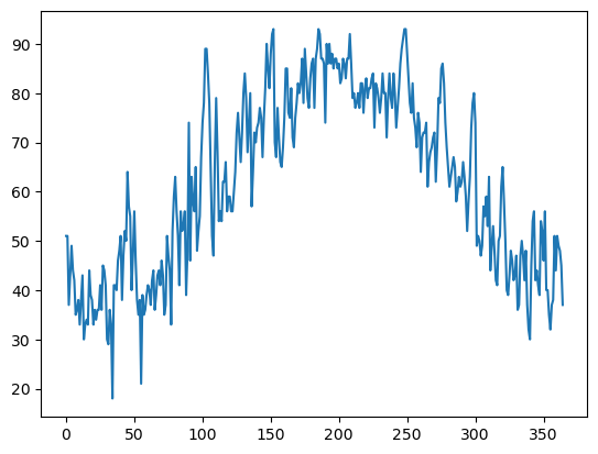
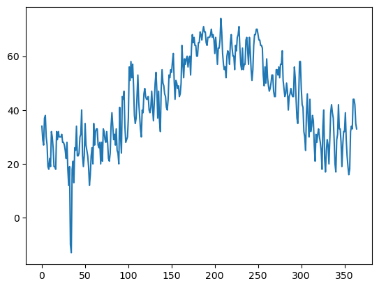
Now let’s visualize the temperature trace over the year! Pandas has a method that directly calls Matplotlib’s plotting package.
maxT.plot()
<Axes: >
minT.plot()
<Axes: >
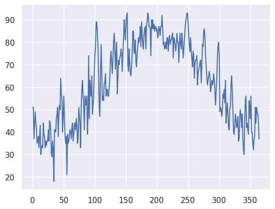
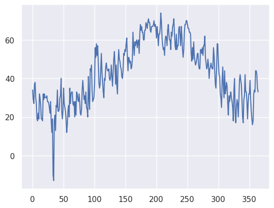
The data plotted fine, but the look could be better. First, let’s import a package, seaborn, that when imported and set using its own method, makes matplotlib’s graphs look better.
Info on seaborn: https://seaborn.pydata.org/index.html
import seaborn as sns
sns.set()
maxT.plot()
<Axes: >
minT.plot()
<Axes: >
Next, let’s plot the two traces simultaneously on the graph so we can better discern max and min temps (this will also enure a single y-axis that will encompass the range of temperature values). We’ll also add some helpful labels and expand the size of the figure.
fig, ax = plt.subplots(figsize=(15,10))
ax.plot (Date, maxT, color='red')
ax.plot (Date, minT, color='blue')
ax.set_title ("ALB Year 2023")
ax.set_xlabel('Day of Year')
ax.set_ylabel('Temperature (°F')
Text(0, 0.5, 'Temperature (°F')
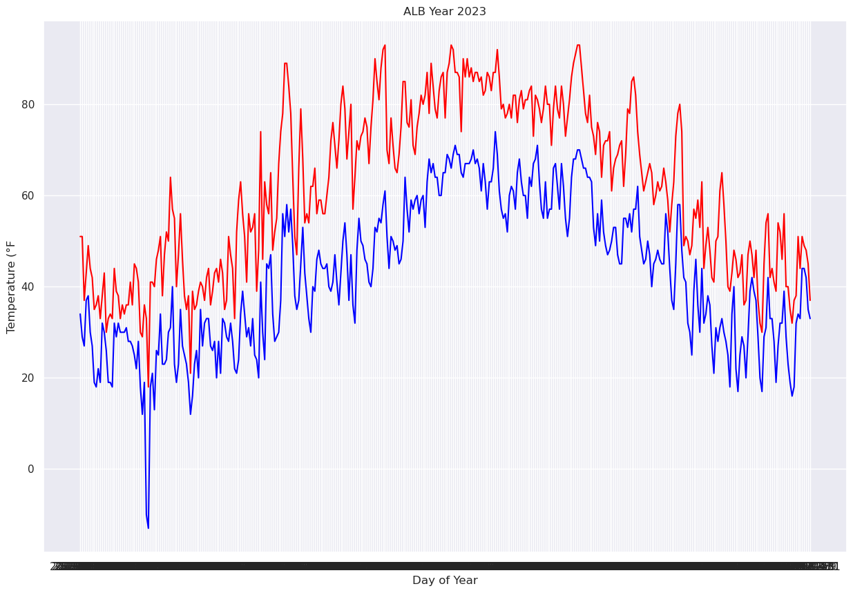
You will notice that this graphic took some time to render. Note that the x-axis label is virtually unreadable. This is because every date is being printed!
We will deal with this by using one of Pandas’ methods that take strings and convert them to a special type of data … not strings nor numbers, but datetime objects. Note carefully how we do this here … it is not terribly intuitive, but we’ll explain it more in an upcoming lecture/notebook on datetime. You will see though that the output column now looks a bit more date-like, with a four-digit year followed by two-digit month and date.
Date = pd.to_datetime(Date,format="%Y-%m-%d")
Date
0     2023-01-01
1     2023-01-02
2     2023-01-03
3     2023-01-04
4     2023-01-05
5     2023-01-06
6     2023-01-07
7     2023-01-08
8     2023-01-09
9     2023-01-10
10    2023-01-11
11    2023-01-12
12    2023-01-13
13    2023-01-14
14    2023-01-15
15    2023-01-16
16    2023-01-17
17    2023-01-18
18    2023-01-19
19    2023-01-20
20    2023-01-21
21    2023-01-22
22    2023-01-23
23    2023-01-24
24    2023-01-25
25    2023-01-26
26    2023-01-27
27    2023-01-28
28    2023-01-29
29    2023-01-30
30    2023-01-31
31    2023-02-01
32    2023-02-02
33    2023-02-03
34    2023-02-04
35    2023-02-05
36    2023-02-06
37    2023-02-07
38    2023-02-08
39    2023-02-09
40    2023-02-10
41    2023-02-11
42    2023-02-12
43    2023-02-13
44    2023-02-14
45    2023-02-15
46    2023-02-16
47    2023-02-17
48    2023-02-18
49    2023-02-19
50    2023-02-20
51    2023-02-21
52    2023-02-22
53    2023-02-23
54    2023-02-24
55    2023-02-25
56    2023-02-26
57    2023-02-27
58    2023-02-28
59    2023-03-01
60    2023-03-02
61    2023-03-03
62    2023-03-04
63    2023-03-05
64    2023-03-06
65    2023-03-07
66    2023-03-08
67    2023-03-09
68    2023-03-10
69    2023-03-11
70    2023-03-12
71    2023-03-13
72    2023-03-14
73    2023-03-15
74    2023-03-16
75    2023-03-17
76    2023-03-18
77    2023-03-19
78    2023-03-20
79    2023-03-21
80    2023-03-22
81    2023-03-23
82    2023-03-24
83    2023-03-25
84    2023-03-26
85    2023-03-27
86    2023-03-28
87    2023-03-29
88    2023-03-30
89    2023-03-31
90    2023-04-01
91    2023-04-02
92    2023-04-03
93    2023-04-04
94    2023-04-05
95    2023-04-06
96    2023-04-07
97    2023-04-08
98    2023-04-09
99    2023-04-10
100   2023-04-11
101   2023-04-12
102   2023-04-13
103   2023-04-14
104   2023-04-15
105   2023-04-16
106   2023-04-17
107   2023-04-18
108   2023-04-19
109   2023-04-20
110   2023-04-21
111   2023-04-22
112   2023-04-23
113   2023-04-24
114   2023-04-25
115   2023-04-26
116   2023-04-27
117   2023-04-28
118   2023-04-29
119   2023-04-30
120   2023-05-01
121   2023-05-02
122   2023-05-03
123   2023-05-04
124   2023-05-05
125   2023-05-06
126   2023-05-07
127   2023-05-08
128   2023-05-09
129   2023-05-10
130   2023-05-11
131   2023-05-12
132   2023-05-13
133   2023-05-14
134   2023-05-15
135   2023-05-16
136   2023-05-17
137   2023-05-18
138   2023-05-19
139   2023-05-20
140   2023-05-21
141   2023-05-22
142   2023-05-23
143   2023-05-24
144   2023-05-25
145   2023-05-26
146   2023-05-27
147   2023-05-28
148   2023-05-29
149   2023-05-30
150   2023-05-31
151   2023-06-01
152   2023-06-02
153   2023-06-03
154   2023-06-04
155   2023-06-05
156   2023-06-06
157   2023-06-07
158   2023-06-08
159   2023-06-09
160   2023-06-10
161   2023-06-11
162   2023-06-12
163   2023-06-13
164   2023-06-14
165   2023-06-15
166   2023-06-16
167   2023-06-17
168   2023-06-18
169   2023-06-19
170   2023-06-20
171   2023-06-21
172   2023-06-22
173   2023-06-23
174   2023-06-24
175   2023-06-25
176   2023-06-26
177   2023-06-27
178   2023-06-28
179   2023-06-29
180   2023-06-30
181   2023-07-01
182   2023-07-02
183   2023-07-03
184   2023-07-04
185   2023-07-05
186   2023-07-06
187   2023-07-07
188   2023-07-08
189   2023-07-09
190   2023-07-10
191   2023-07-11
192   2023-07-12
193   2023-07-13
194   2023-07-14
195   2023-07-15
196   2023-07-16
197   2023-07-17
198   2023-07-18
199   2023-07-19
200   2023-07-20
201   2023-07-21
202   2023-07-22
203   2023-07-23
204   2023-07-24
205   2023-07-25
206   2023-07-26
207   2023-07-27
208   2023-07-28
209   2023-07-29
210   2023-07-30
211   2023-07-31
212   2023-08-01
213   2023-08-02
214   2023-08-03
215   2023-08-04
216   2023-08-05
217   2023-08-06
218   2023-08-07
219   2023-08-08
220   2023-08-09
221   2023-08-10
222   2023-08-11
223   2023-08-12
224   2023-08-13
225   2023-08-14
226   2023-08-15
227   2023-08-16
228   2023-08-17
229   2023-08-18
230   2023-08-19
231   2023-08-20
232   2023-08-21
233   2023-08-22
234   2023-08-23
235   2023-08-24
236   2023-08-25
237   2023-08-26
238   2023-08-27
239   2023-08-28
240   2023-08-29
241   2023-08-30
242   2023-08-31
243   2023-09-01
244   2023-09-02
245   2023-09-03
246   2023-09-04
247   2023-09-05
248   2023-09-06
249   2023-09-07
250   2023-09-08
251   2023-09-09
252   2023-09-10
253   2023-09-11
254   2023-09-12
255   2023-09-13
256   2023-09-14
257   2023-09-15
258   2023-09-16
259   2023-09-17
260   2023-09-18
261   2023-09-19
262   2023-09-20
263   2023-09-21
264   2023-09-22
265   2023-09-23
266   2023-09-24
267   2023-09-25
268   2023-09-26
269   2023-09-27
270   2023-09-28
271   2023-09-29
272   2023-09-30
273   2023-10-01
274   2023-10-02
275   2023-10-03
276   2023-10-04
277   2023-10-05
278   2023-10-06
279   2023-10-07
280   2023-10-08
281   2023-10-09
282   2023-10-10
283   2023-10-11
284   2023-10-12
285   2023-10-13
286   2023-10-14
287   2023-10-15
288   2023-10-16
289   2023-10-17
290   2023-10-18
291   2023-10-19
292   2023-10-20
293   2023-10-21
294   2023-10-22
295   2023-10-23
296   2023-10-24
297   2023-10-25
298   2023-10-26
299   2023-10-27
300   2023-10-28
301   2023-10-29
302   2023-10-30
303   2023-10-31
304   2023-11-01
305   2023-11-02
306   2023-11-03
307   2023-11-04
308   2023-11-05
309   2023-11-06
310   2023-11-07
311   2023-11-08
312   2023-11-09
313   2023-11-10
314   2023-11-11
315   2023-11-12
316   2023-11-13
317   2023-11-14
318   2023-11-15
319   2023-11-16
320   2023-11-17
321   2023-11-18
322   2023-11-19
323   2023-11-20
324   2023-11-21
325   2023-11-22
326   2023-11-23
327   2023-11-24
328   2023-11-25
329   2023-11-26
330   2023-11-27
331   2023-11-28
332   2023-11-29
333   2023-11-30
334   2023-12-01
335   2023-12-02
336   2023-12-03
337   2023-12-04
338   2023-12-05
339   2023-12-06
340   2023-12-07
341   2023-12-08
342   2023-12-09
343   2023-12-10
344   2023-12-11
345   2023-12-12
346   2023-12-13
347   2023-12-14
348   2023-12-15
349   2023-12-16
350   2023-12-17
351   2023-12-18
352   2023-12-19
353   2023-12-20
354   2023-12-21
355   2023-12-22
356   2023-12-23
357   2023-12-24
358   2023-12-25
359   2023-12-26
360   2023-12-27
361   2023-12-28
362   2023-12-29
363   2023-12-30
364   2023-12-31
Name: DATE, dtype: datetime64[ns]
Matplotlib will recognize this array as being date/time-related, and when we pass it in as the x-axis, the graphic appears faster, and we also have a more meaningful x-axis label.
fig, ax = plt.subplots(figsize=(15,10))
ax.plot (Date, maxT, color='red')
ax.plot (Date, minT, color='blue')
ax.set_title ("ALB Year 2023")
ax.set_xlabel('Day of Year')
ax.set_ylabel('Temperature (°F)')
Text(0, 0.5, 'Temperature (°F)')
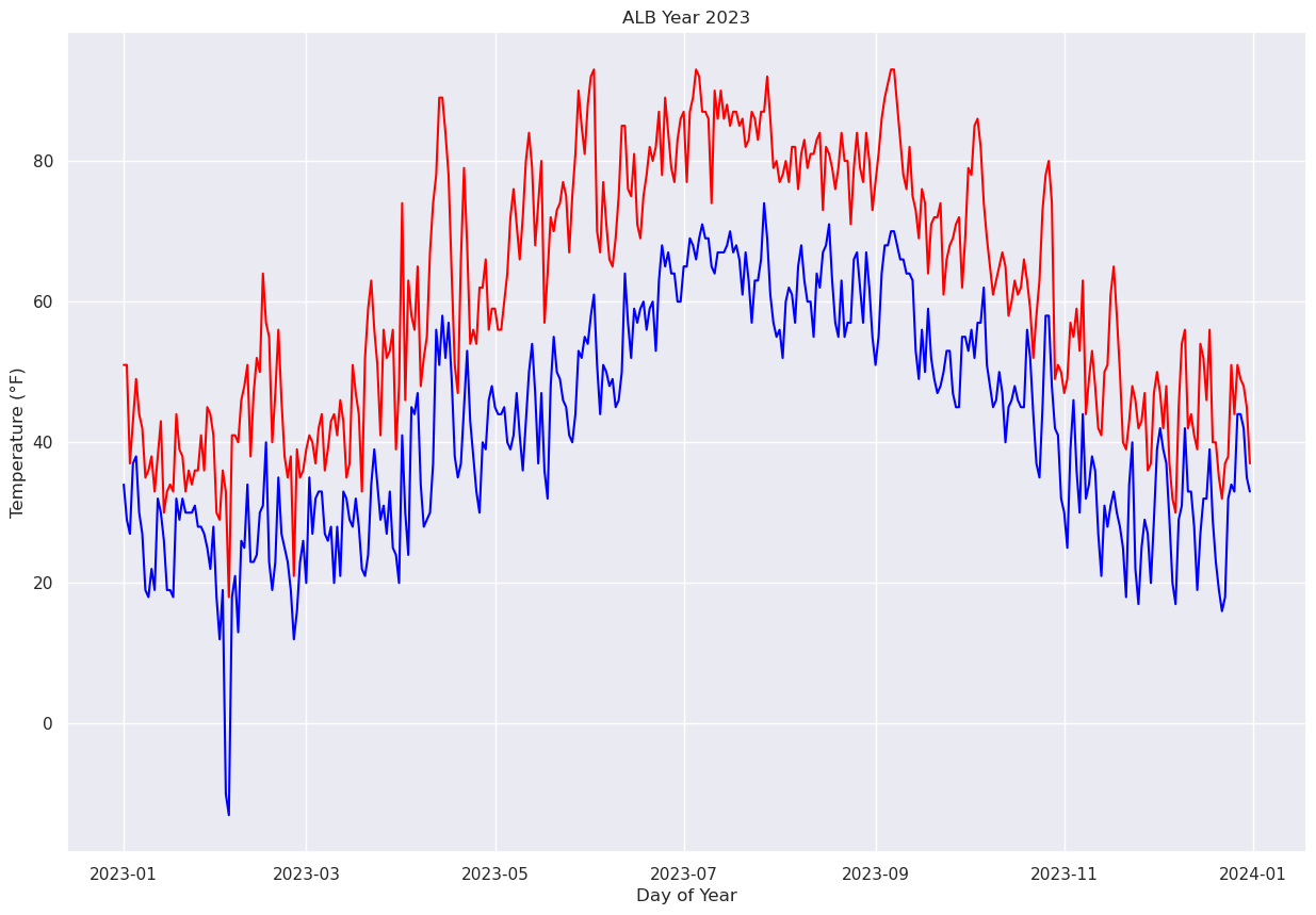
We’ll further refine the look of the plot by adding a legend and have vertical grid lines on a frequency of one month.
from matplotlib.dates import DateFormatter, AutoDateLocator,HourLocator,DayLocator,MonthLocator
fig, ax = plt.subplots(figsize=(15,10))
ax.plot (Date, maxT, color='red',label = "Max T")
ax.plot (Date, minT, color='blue', label = "Min T")
ax.set_title ("ALB Year 2023")
ax.set_xlabel('Date')
ax.set_ylabel('Temperature (°F)' )
ax.xaxis.set_major_locator(MonthLocator(interval=1))
dateFmt = DateFormatter('%b %d')
ax.xaxis.set_major_formatter(dateFmt)
ax.legend (loc="best")
<matplotlib.legend.Legend at 0x154267d66690>
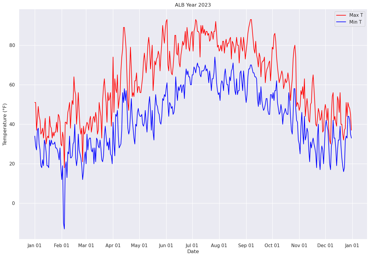
Let’s save our beautiful graphic to disk.
fig.savefig ('albTemps2023.png')
Now, let’s answer the question, “what was the most common range of maximum temperatures last year in Albany?” via a histogram. We use matplotlib’s hist method.
# Create a figure and size it.
fig, ax = plt.subplots(figsize=(15,10))
# Create a histogram of our data series and divide it in to 10 bins.
ax.hist(maxT, bins=10, color='k', alpha=0.3)
(array([ 2.,  6., 49., 47., 43., 33., 39., 46., 62., 38.]),
 array([18. , 25.5, 33. , 40.5, 48. , 55.5, 63. , 70.5, 78. , 85.5, 93. ]),
 <BarContainer object of 10 artists>)
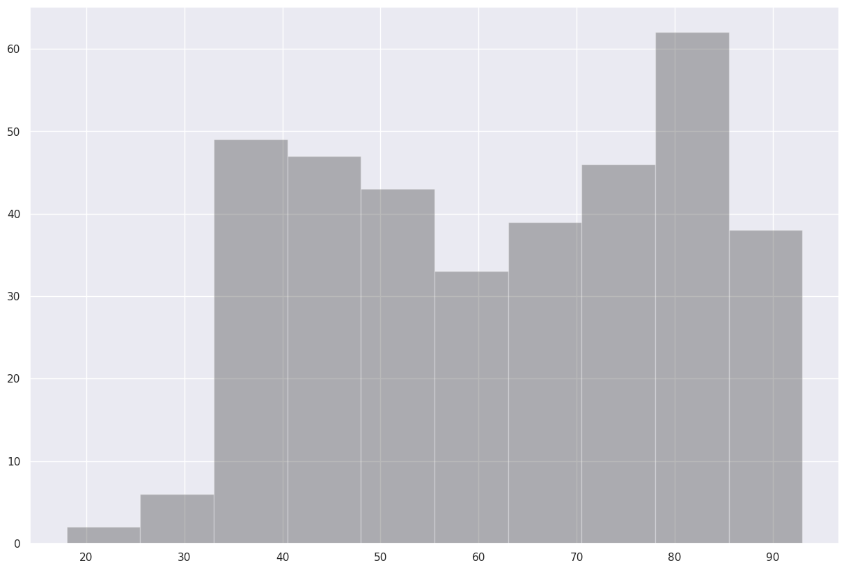
Ok, but the 10 bins were autoselected. Let’s customize our call to the hist method by specifying the bounds of each of our bins.
How can we learn more about how to customize this call? Append a ? to the name of the method.
ax.hist?
Revise the call to ax.hist, and also draw tick marks that align with the bounds of the histogram’s bins.
fig, ax = plt.subplots(figsize=(15,10))
ax.hist(maxT, bins=(0,10,20,30,40,50,60,70,80,90,100), color='k', alpha=0.3)
ax.xaxis.set_major_locator(plt.MultipleLocator(10))
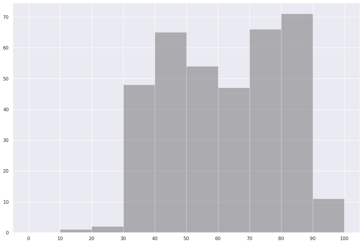
Save this histogram to disk.
fig.savefig("maxT_hist.png")
Use the describe method on the maximum temperature series to reveal some simple statistical properties.
maxT.describe()
count    365.000000
mean      61.879452
std       18.183035
min       18.000000
25%       46.000000
50%       63.000000
75%       79.000000
max       93.000000
Name: MAX, dtype: float64