Pandas 3: Plotting NYS Mesonet Observations¶

Overview¶

In this notebook, we’ll use Pandas to read in and analyze current data from the New York State Mesonet. We will also use Matplotlib to plot the locations of NYSM sites.

Prerequisites¶

Concepts	Importance	Notes
Matplotlib	Necessary
Pandas	Necessary

Time to learn: 15 minutes

Imports¶

import matplotlib.pyplot as plt
import numpy as np
import pandas as pd

Create a Pandas DataFrame object pointing to the latest set of obs.

nysm_data = pd.read_csv('https://www.atmos.albany.edu/products/nysm/nysm_latest.csv')

Create Series objects for several columns from the DataFrame.

First, remind ourselves of the column names.

nysm_data.columns

Index(['station', 'time', 'temp_2m [degC]', 'temp_9m [degC]',
       'relative_humidity [percent]', 'precip_incremental [mm]',
       'precip_local [mm]', 'precip_max_intensity [mm/min]',
       'avg_wind_speed_prop [m/s]', 'max_wind_speed_prop [m/s]',
       'wind_speed_stddev_prop [m/s]', 'wind_direction_prop [degrees]',
       'wind_direction_stddev_prop [degrees]', 'avg_wind_speed_sonic [m/s]',
       'max_wind_speed_sonic [m/s]', 'wind_speed_stddev_sonic [m/s]',
       'wind_direction_sonic [degrees]',
       'wind_direction_stddev_sonic [degrees]', 'solar_insolation [W/m^2]',
       'station_pressure [mbar]', 'snow_depth [cm]', 'frozen_soil_05cm [bit]',
       'frozen_soil_25cm [bit]', 'frozen_soil_50cm [bit]',
       'soil_temp_05cm [degC]', 'soil_temp_25cm [degC]',
       'soil_temp_50cm [degC]', 'soil_moisture_05cm [m^3/m^3]',
       'soil_moisture_25cm [m^3/m^3]', 'soil_moisture_50cm [m^3/m^3]', 'lat',
       'lon', 'elevation', 'name'],
      dtype='object')

Create several Series objects for particular columns of interest.

stid = nysm_data['station']
lats = nysm_data['lat']
lons = nysm_data['lon']
time = nysm_data['time']
tmpc = nysm_data['temp_2m [degC]']
tmpc9 = nysm_data['temp_9m [degC]']
rh   = nysm_data['relative_humidity [percent]']
pres = nysm_data['station_pressure [mbar]']
wspd = nysm_data['max_wind_speed_prop [m/s]']
drct = nysm_data['wind_direction_prop [degrees]']
pinc = nysm_data['precip_incremental [mm]']
ptot = nysm_data['precip_local [mm]']
pint = nysm_data['precip_max_intensity [mm/min]']

Examine one or more of these Series.

tmpc

    16.5
    18.6
    11.8
    17.6
    19.4
       ... 
   5.3
  13.3
  10.3
  10.7
  14.0
Name: temp_2m [degC], Length: 126, dtype: float64

Exercise: Read in at least one additional Series object.

# Write your code below

Tip: Each of these Series objects contain data stored as NumPy arrays. As a result, we can take advantage of vectorizing, which perform operations on all array elements without needing to construct a Python for loop.

Convert the temperature and wind speed arrays to Fahrenheit and knots, respectively.

tmpf = tmpc * 1.8 + 32
wspk = wspd * 1.94384

Examine the new Series. Note that every element of the array has been calculated using the arithemtic above … in just one line of code per Series!

tmpf

    61.70
    65.48
    53.24
    63.68
    66.92
       ...  
  41.54
  55.94
  50.54
  51.26
  57.20
Name: temp_2m [degC], Length: 126, dtype: float64

Note: The metadata did not change to reflect the change in units! That is something we'd have to change manually, via the Series' name attribute.

tmpf.name = 'temp_2m [degF]'

tmpf

    61.70
    65.48
    53.24
    63.68
    66.92
       ...  
  41.54
  55.94
  50.54
  51.26
  57.20
Name: temp_2m [degF], Length: 126, dtype: float64

Next, get the basic statistical properties of one of the Series.

tmpf.describe()

count    126.000000
mean      57.021429
std        6.327792
min       41.360000
25%       51.440000
50%       56.930000
75%       62.645000
max       69.980000
Name: temp_2m [degF], dtype: float64

Exercise: Convert the 9-m temperature to Fahrenheit, and examine its corresponding statistical properties. What do you notice in terms of the count? Why is there a difference in counts between the 9 m and 2 m arrays?

# Write your code below

Plot station locations using Matplotlib¶

We use another plotting method for an Axes element … in this case, a Scatter plot. We pass as arguments into this method the x- and y-arrays, corresponding to longitudes and latitudes, and then set five additional attributes.

fig = plt.figure(figsize=(12,9))
ax = fig.add_subplot(1,1,1)
ax.set_title ('New York State Mesonet Site Locations')
ax.scatter(lons,lats,s=9,c='r',edgecolor='black',alpha=0.75)

<matplotlib.collections.PathCollection at 0x15052a3b5550>

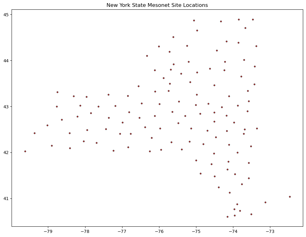
../../_images/9ce2c0df6f1401562380383451695f520bc5cd6fa77a3155be2dcd53124e3ee4.png

Exercise: Examine the link above for how we can call the scatter function. Try changing one or more of the five argument values we used above, and try different arguments as well.

What’s Next?¶

We can discern the outline of New York State! But wouldn’t it be nice if we could plot cartographic features, such as physical and/or political borders (e.g., coastlines, national/state/provincial boundaries), as well as georeference the data we are plotting? We’ll cover that next with the Cartopy package!

ATM350 Spring 2024

Pandas 3: Plotting NYS Mesonet Observations

Contents