Skew-T’s
Contents
Skew-T’s
Use functions to loop over dates and stations
Demonstrate Python’s try ... except utility
Import the libraries we need
import numpy as np
import matplotlib.pyplot as plt
from mpl_toolkits.axes_grid1.inset_locator import inset_axes
import metpy.calc as mpcalc
from metpy.plots import Hodograph, SkewT
from metpy.units import units, pandas_dataframe_to_unit_arrays
from datetime import datetime, timedelta
from dateutil.relativedelta import relativedelta
from time import sleep
import pandas as pd
from siphon.simplewebservice.wyoming import WyomingUpperAir
Define a function that will retrieve the skew-t from the Wyoming data server.
def retrieveSkewt (t, site):
    '''
    This function obtains sounding data for a particular time and location, and draws a Skew-T
    '''

    curtim = t.strftime("%y%m%d%H")
    print (f"Processing {t} for {site}")

#   Query the UWyoming Data Server. Handle the situation when a data retrieval error occurs.
    try:
        df = WyomingUpperAir.request_data (t ,site)
        drawSkewt(df, site, current, lev)
    except Exception as errorMsg:
        print (f"Error returning sounding for {site} at {t}: {errorMsg}")
Define a function that will process and draw the skew-t from the Wyoming data server.
def drawSkewt(df, site, dattim, lev):
'''
drawSkewt processes and draws a Skew-t that has been downloaded from the UWyoming server.
'''
raob_timeStr = dattim.strftime("%Y%m%d%H")
raob_timeTitle = dattim.strftime("%H00 UTC %-d %b %Y")
### Attach units to the various columns using MetPy's `pandas_dataframe_to_unit_arrays` function, as follows:
df = pandas_dataframe_to_unit_arrays(df)
# As with any Pandas Dataframe, we can select columns, so we do so now for all the relevant variables for our Skew-T.
P = df['pressure']
Z = df['height']
T = df['temperature']
Td = df['dewpoint']
U = df['u_wind']
V = df['v_wind']
# Now that U and V are units aware, we can use one of MetPy's diagnostic routines to
# calculate the wind speed from the vector's components.
wind_speed = mpcalc.wind_speed(U, V)
# Calculate the LCL
lclp, lclt = mpcalc.lcl(P[lev], T[lev], Td[lev])
# Calculate the parcel profile. Here, we pass in the array of all pressure values, and specify the index of the temperature and dewpoint arrays as the starting point of the parcel path.
parcel_prof = mpcalc.parcel_profile(P[lev:], T[lev], Td[lev])
# Set the limits for the x- and y-axes so they can be changed and easily re-used when desired.
pTop = 100
pBot = 1050
tMin = -60
tMax = 40
# Define the log-p axis.
logTop = np.log10(pTop)
logBot = np.log10(pBot)
interval = np.logspace(logTop,logBot) * units('hPa')
# This interval will tend to oversample points near the top of the atmosphere relative to the bottom.
# One effect of this will be that wind barbs will be hard to read, especially at higher levels.
# Use a resampling method from NumPy to deal with this.
idx = mpcalc.resample_nn_1d(P, interval)
# Plot the skew-t and save it as a PNG file.
# Create a new figure. The dimensions here give a good aspect ratio
fig = plt.figure(figsize=(9, 9))
skew = SkewT(fig, rotation=30)
# Plot the data using normal plotting functions, in this case using
# log scaling in Y, as dictated by the typical meteorological plot
skew.plot(P, T, 'r', linewidth=3)
skew.plot(P, Td, 'g', linewidth=3)
skew.plot_barbs(P[idx],U[idx], V[idx])
skew.ax.set_ylim(pBot, pTop)
skew.ax.set_xlim(tMin, tMax)
# Plot LCL as black dot
skew.plot(lclp, lclt, 'ko', markerfacecolor='black')
# Plot the parcel profile as a black line
skew.plot(P[lev:], parcel_prof, 'k', linestyle='--', linewidth=2)
# Shade areas of CAPE and CIN
skew.shade_cin(P[lev:], T[lev:], parcel_prof)
skew.shade_cape(P[lev:], T[lev:], parcel_prof)
# Shade areas between a certain temperature (in this case, the DGZ)
skew.shade_area(P.m,-18,-12,color=['purple'])
# Plot a zero degree isotherm
skew.ax.axvline(0, color='c', linestyle='-', linewidth=2)
# Add the relevant special lines
skew.plot_dry_adiabats()
skew.plot_moist_adiabats(colors='#58a358', linestyle='-')
skew.plot_mixing_lines()
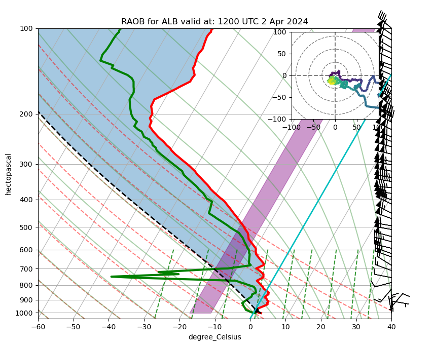
plt.title(f"RAOB for {station} valid at: {raob_timeTitle}")
# Create a hodograph
# Create an inset axes object that is 30% width and height of the
# figure and put it in the upper right hand corner.
ax_hod = inset_axes(skew.ax, '30%', '30%', loc=1)
h = Hodograph(ax_hod, component_range=100.)
h.add_grid(increment=30)
h.plot_colormapped(U, V, df['height'])
plt.savefig (f"{site}_{raob_timeStr}_skewt.png")
Set the stations, and the date/time range over which you wish to produce skew-t’s.
stationList = ['ALB', 'BUF']
stationList = ['ALB']
start = datetime(2024,4,2,12)

end = datetime(2024,4,2,12)
Set the level from which you wish to raise the parcel from (0 = lowest level)
lev = 0
Loop over the times; retrieve and draw the Skew-t
current = start

while (current <= end):
    for station in stationList:
        # Sleep 5 seconds as an attempt to avoid UWyoming 503 Server Busy errors
        sleep(5)
        df = retrieveSkewt(current, station)
        current = current + relativedelta(hours=12)
Processing 2024-04-02 12:00:00 for ALB
Possible data retrieval errors:
- You may have specified an incorrect date or location, or there just might not have been a successful RAOB at that date and time.
- The Wyoming server does not handle simultaneous requests well. If indeed there was a sounding taken for the site and time, usually the request will eventually work.
Things to try:
- Basic: Modify the stations and times to fit your final project
- Basic: Use comment lines to modify the
drawSkewtfunction to change or omit what's drawn on the Skew-t (e.g., omit the DGZ if irrelevant to your case) - Advanced: Modify the
drawSkewtfunction so what's drawn or omitted on the Skew-t is passed as an argument (hint: use a dictionary) - Advanced: Refine the
retrieveSkewtfunction so error exceptions are handled better (e.g., automatically attempt to retrieve a sounding if a prior attempt fails with a503error - Advanced: Specify a particular pressure level, rather than a row index, and for each sounding, find the row index that is closest to the specified pressure value