Meteogram
Contents
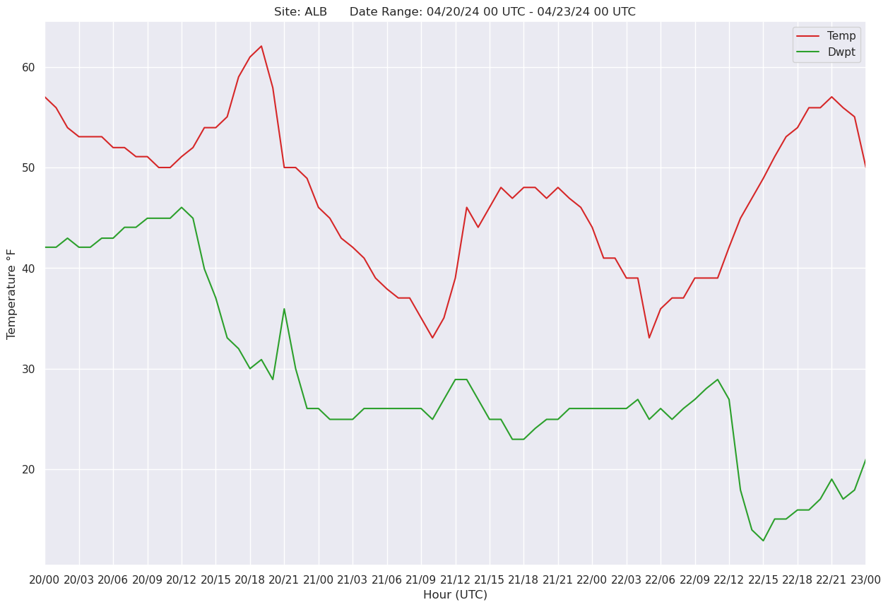
Meteogram
Here we draw a surface meteogram, from data that we retrieve from our METAR archive.
Imports
import numpy as np
import pandas as pd

import matplotlib.pyplot as plt
from matplotlib.dates import DateFormatter, AutoDateLocator,YearLocator, HourLocator,DayLocator,MonthLocator

from metpy.units import units
from datetime import datetime, timedelta
import seaborn as sns
Set the desired start and end time (UTC), and create strings for the figure title.
startTime = datetime(2024,4,20,0)
endTime = datetime(2024,4,23,0)
sTimeStr = startTime.strftime(format="%x %H UTC")
eTimeStr = endTime.strftime(format="%x %H UTC")
Create an empty Dateframe to which we will concatenate the hourly CSV files in the desired time range.
df = pd.DataFrame()
Loop over each hour. Concatenate each hour’s METARs into the full Dataframe.
curTime = startTime
while (curTime <= endTime):
    print (curTime)
    timeStr = curTime.strftime("%y%m%d%H")
    metarCSV = f'/ktyle_rit/scripts/sflist2/complete/{timeStr}.csv'
    dfTemp = pd.read_csv(metarCSV, sep='\s+')
    df = pd.concat([df, dfTemp], ignore_index=True)
    curTime = curTime + timedelta(hours=1)
2024-04-20 00:00:00
2024-04-20 01:00:00
2024-04-20 02:00:00
2024-04-20 03:00:00
2024-04-20 04:00:00
2024-04-20 05:00:00
2024-04-20 06:00:00
2024-04-20 07:00:00
2024-04-20 08:00:00
2024-04-20 09:00:00
2024-04-20 10:00:00
2024-04-20 11:00:00
2024-04-20 12:00:00
2024-04-20 13:00:00
2024-04-20 14:00:00
2024-04-20 15:00:00
2024-04-20 16:00:00
2024-04-20 17:00:00
2024-04-20 18:00:00
2024-04-20 19:00:00
2024-04-20 20:00:00
2024-04-20 21:00:00
2024-04-20 22:00:00
2024-04-20 23:00:00
2024-04-21 00:00:00
2024-04-21 01:00:00
2024-04-21 02:00:00
2024-04-21 03:00:00
2024-04-21 04:00:00
2024-04-21 05:00:00
2024-04-21 06:00:00
2024-04-21 07:00:00
2024-04-21 08:00:00
2024-04-21 09:00:00
2024-04-21 10:00:00
2024-04-21 11:00:00
2024-04-21 12:00:00
2024-04-21 13:00:00
2024-04-21 14:00:00
2024-04-21 15:00:00
2024-04-21 16:00:00
2024-04-21 17:00:00
2024-04-21 18:00:00
2024-04-21 19:00:00
2024-04-21 20:00:00
2024-04-21 21:00:00
2024-04-21 22:00:00
2024-04-21 23:00:00
2024-04-22 00:00:00
2024-04-22 01:00:00
2024-04-22 02:00:00
2024-04-22 03:00:00
2024-04-22 04:00:00
2024-04-22 05:00:00
2024-04-22 06:00:00
2024-04-22 07:00:00
2024-04-22 08:00:00
2024-04-22 09:00:00
2024-04-22 10:00:00
2024-04-22 11:00:00
2024-04-22 12:00:00
2024-04-22 13:00:00
2024-04-22 14:00:00
2024-04-22 15:00:00
2024-04-22 16:00:00
2024-04-22 17:00:00
2024-04-22 18:00:00
2024-04-22 19:00:00
2024-04-22 20:00:00
2024-04-22 21:00:00
2024-04-22 22:00:00
2024-04-22 23:00:00
2024-04-23 00:00:00
Examine the Dataframe
df
| STN | YYMMDD/HHMM | SLAT | SLON | SELV | PMSL | ALTI | TMPC | DWPC | SKNT | ... | P03C | CTYL | CTYM | CTYH | P06I | T6XC | T6NC | CEIL | P01I | SNEW | |
|---|---|---|---|---|---|---|---|---|---|---|---|---|---|---|---|---|---|---|---|---|---|
| 0 | DYS | 240420/0000 | 32.43 | -99.85 | 545.0 | 1014.0 | 30.01 | 18.0 | 9.3 | 10.0 | ... | -1.2 | -9999.0 | -9999.0 | -9999.0 | -9999.0 | 18.3 | 14.4 | 27.0 | -9999.0 | -9999.0 |
| 1 | NUW | 240420/0000 | 48.35 | -122.65 | 14.0 | 1020.5 | 30.13 | 15.6 | 2.8 | 6.0 | ... | -1.6 | -9999.0 | -9999.0 | -9999.0 | -9999.0 | 17.2 | 13.3 | -9999.0 | -9999.0 | -9999.0 |
| 2 | NYL | 240420/0000 | 32.65 | -114.62 | 65.0 | 1005.9 | 29.71 | 32.8 | -0.6 | 6.0 | ... | -1.8 | -9999.0 | -9999.0 | -9999.0 | -9999.0 | 32.8 | 28.3 | -9999.0 | -9999.0 | -9999.0 |
| 3 | PALU | 240420/0000 | 68.88 | -166.13 | 3.0 | 1022.8 | 30.21 | -4.8 | -8.2 | 24.0 | ... | 1.5 | -9999.0 | -9999.0 | -9999.0 | -9999.0 | -4.8 | -8.6 | -9999.0 | -9999.0 | -9999.0 |
| 4 | PATC | 240420/0000 | 65.57 | -167.92 | 83.0 | 1021.1 | 30.13 | -9.8 | -12.3 | 21.0 | ... | -0.5 | -9999.0 | -9999.0 | -9999.0 | -9999.0 | -9.4 | -13.7 | 110.0 | -9999.0 | -9999.0 |
| ... | ... | ... | ... | ... | ... | ... | ... | ... | ... | ... | ... | ... | ... | ... | ... | ... | ... | ... | ... | ... | ... |
| 314571 | K70 | 240423/0000 | -9999.00 | -9999.00 | -9999.0 | -9999.0 | 29.95 | 25.0 | 22.0 | 10.0 | ... | -9999.0 | -9999.0 | -9999.0 | -9999.0 | -9999.0 | -9999.0 | -9999.0 | 39.0 | -9999.0 | -9999.0 |
| 314572 | EKE | 240423/0000 | -9999.00 | -9999.00 | -9999.0 | -9999.0 | 30.08 | 18.0 | 7.0 | 13.0 | ... | -9999.0 | -9999.0 | -9999.0 | -9999.0 | -9999.0 | -9999.0 | -9999.0 | -9999.0 | -9999.0 | -9999.0 |
| 314573 | EZP | 240423/0000 | -9999.00 | -9999.00 | -9999.0 | -9999.0 | 30.13 | 19.0 | 11.0 | 15.0 | ... | -9999.0 | -9999.0 | -9999.0 | -9999.0 | -9999.0 | -9999.0 | -9999.0 | -9999.0 | -9999.0 | -9999.0 |
| 314574 | F45 | 240423/0000 | -9999.00 | -9999.00 | -9999.0 | -9999.0 | 30.01 | 20.0 | 17.0 | 11.0 | ... | -9999.0 | -9999.0 | -9999.0 | -9999.0 | -9999.0 | -9999.0 | -9999.0 | 60.0 | -9999.0 | -9999.0 |
| 314575 | 0R4 | 240423/0000 | -9999.00 | -9999.00 | -9999.0 | -9999.0 | 30.18 | 19.3 | 2.9 | 3.0 | ... | -9999.0 | -9999.0 | -9999.0 | -9999.0 | -9999.0 | 20.3 | 17.7 | -9999.0 | -9999.0 | -9999.0 |
314576 rows × 35 columns
Select the station from which to subset the Dataframe.
site = 'ALB'
Create a new Dataframe that contains only the rows for the desired site.
dfSub = df.query('STN == @site')
Create a new column that represents the date and time as a datetime64 object.
# Next line suppresses a warning message. See https://pandas.pydata.org/pandas-docs/stable/user_guide/indexing.html#returning-a-view-versus-a-copy.
# This won't be necessary with Pandas version 3 and beyond.

pd.options.mode.copy_on_write = True

dattim = pd.to_datetime(dfSub['YYMMDD/HHMM'],format="%y%m%d/%H%M", utc=True)
dfSub['DATETIME'] = dattim
Examine the subsetted Dataframe.
dfSub
| STN | YYMMDD/HHMM | SLAT | SLON | SELV | PMSL | ALTI | TMPC | DWPC | SKNT | ... | CTYL | CTYM | CTYH | P06I | T6XC | T6NC | CEIL | P01I | SNEW | DATETIME | |
|---|---|---|---|---|---|---|---|---|---|---|---|---|---|---|---|---|---|---|---|---|---|
| 1084 | ALB | 240420/0000 | 42.75 | -73.8 | 89.0 | 1014.9 | 29.97 | 13.9 | 5.6 | 13.0 | ... | -9999.0 | -9999.0 | -9999.0 | 0.0 | 16.7 | 13.3 | 43.0 | -9999.0 | -9999.0 | 2024-04-20 00:00:00+00:00 |
| 5427 | ALB | 240420/0100 | 42.75 | -73.8 | 89.0 | 1015.4 | 29.99 | 13.3 | 5.6 | 12.0 | ... | -9999.0 | -9999.0 | -9999.0 | -9999.0 | -9999.0 | -9999.0 | 39.0 | -9999.0 | -9999.0 | 2024-04-20 01:00:00+00:00 |
| 9721 | ALB | 240420/0200 | 42.75 | -73.8 | 89.0 | 1015.4 | 29.99 | 12.2 | 6.1 | 17.0 | ... | -9999.0 | -9999.0 | -9999.0 | -9999.0 | -9999.0 | -9999.0 | 38.0 | -9999.0 | -9999.0 | 2024-04-20 02:00:00+00:00 |
| 14026 | ALB | 240420/0300 | 42.75 | -73.8 | 89.0 | 1015.5 | 29.99 | 11.7 | 5.6 | 17.0 | ... | -9999.0 | -9999.0 | -9999.0 | -9999.0 | -9999.0 | -9999.0 | 43.0 | -9999.0 | -9999.0 | 2024-04-20 03:00:00+00:00 |
| 18331 | ALB | 240420/0400 | 42.75 | -73.8 | 89.0 | 1014.9 | 29.97 | 11.7 | 5.6 | 14.0 | ... | -9999.0 | -9999.0 | -9999.0 | -9999.0 | -9999.0 | -9999.0 | 38.0 | -9999.0 | -9999.0 | 2024-04-20 04:00:00+00:00 |
| ... | ... | ... | ... | ... | ... | ... | ... | ... | ... | ... | ... | ... | ... | ... | ... | ... | ... | ... | ... | ... | ... |
| 294077 | ALB | 240422/2000 | 42.75 | -73.8 | 89.0 | 1018.3 | 30.07 | 13.3 | -8.3 | 5.0 | ... | -9999.0 | -9999.0 | -9999.0 | -9999.0 | -9999.0 | -9999.0 | -9999.0 | -9999.0 | -9999.0 | 2024-04-22 20:00:00+00:00 |
| 298371 | ALB | 240422/2100 | 42.75 | -73.8 | 89.0 | 1018.2 | 30.06 | 13.9 | -7.2 | 6.0 | ... | -9999.0 | -9999.0 | -9999.0 | -9999.0 | -9999.0 | -9999.0 | -9999.0 | -9999.0 | -9999.0 | 2024-04-22 21:00:00+00:00 |
| 302705 | ALB | 240422/2200 | 42.75 | -73.8 | 89.0 | 1018.4 | 30.07 | 13.3 | -8.3 | 7.0 | ... | -9999.0 | -9999.0 | -9999.0 | -9999.0 | -9999.0 | -9999.0 | -9999.0 | -9999.0 | -9999.0 | 2024-04-22 22:00:00+00:00 |
| 306996 | ALB | 240422/2300 | 42.75 | -73.8 | 89.0 | 1018.5 | 30.07 | 12.8 | -7.8 | 11.0 | ... | -9999.0 | -9999.0 | -9999.0 | -9999.0 | -9999.0 | -9999.0 | -9999.0 | -9999.0 | -9999.0 | 2024-04-22 23:00:00+00:00 |
| 311313 | ALB | 240423/0000 | 42.75 | -73.8 | 89.0 | 1018.7 | 30.08 | 10.0 | -6.1 | 7.0 | ... | -9999.0 | -9999.0 | -9999.0 | -9999.0 | 13.9 | 10.0 | -9999.0 | -9999.0 | -9999.0 | 2024-04-23 00:00:00+00:00 |
73 rows × 36 columns
Select a couple of variables we wish to plot on the meteogram. In this case, 2m temperature and dewpoint.
var1 = dfSub['TMPC']
var2 = dfSub['DWPC']
Examine one of the variables … of course, it’s a Pandas Series.
var1
1084      13.9
5427      13.3
9721      12.2
14026     11.7
18331     11.7
          ...
294077    13.3
298371    13.9
302705    13.3
306996    12.8
311313    10.0
Name: TMPC, Length: 73, dtype: float64
Pandas Series objects don’t support units. We can, however, create Numpy arrays from the Series values attribute and then attach units to them.
tmpc = var1.values * units('degC')
dwpc = var2.values * units('degC')
Examine one of the units-aware arrays.
tmpc
| Magnitude | [13.9 13.3 12.2 11.7 11.7 11.7 11.1 11.1 10.6 10.6 10.0 10.0 10.6 11.1 |
|---|---|
| Units | degree_Celsius |
Now convert into degrees F.
tmpf = tmpc.to('degF')
dwpf = dwpc.to('degF')
Create the meteogram and save the figure to disk.
sns.set()

fig, ax = plt.subplots(figsize=(15, 10))

# Improve on the default ticking

ax.xaxis.set_major_locator(HourLocator(interval=3))
hoursFmt = DateFormatter('%d/%H')
ax.xaxis.set_major_formatter(hoursFmt)

ax.plot(dfSub['DATETIME'], tmpf, color='tab:red', label='Temp')
ax.plot(dfSub['DATETIME'], dwpf, color='tab:green', label='Dwpt')

ax.set_title(f'Site: {site}      Date Range: {sTimeStr} - {eTimeStr}')

ax.set_xlabel('Hour (UTC)')
ax.set_ylabel('Temperature °F')
ax.set_xlim(startTime, endTime)
ax.legend(loc='best')

fig.savefig (f'{site}_mgram.png')
Things to try:
- Basic Select a site and time range relevant for your case
- Basic Create a multi-panel figure, each displaying a variable of interest
- Advanced Plot two variables that have different units; create corresponding y-axis labels on the left and right sides of the plot