ATM 433/533 Week 1 Sample Notebook
Contents
ATM 433/533 Week 1 Sample Notebook
This is an example Jupyter notebook that uses built-in Python functions, as well as external packages such as Cartopy, Matplotlib, Datetime, MetPy, and Pandas to visualize data from the New York State Mesonet, headquartered right here at UAlbany.
Import the necessary libraries
import matplotlib.pyplot as plt
import numpy as np
import pandas as pd
from datetime import datetime
from cartopy import crs as ccrs
from cartopy import feature as cfeature
from metpy.calc import wind_components
from metpy.units import units
from metpy.plots import StationPlot
Specify the format of the date/time string that is used in the NYSM data files
timeFormat = "%Y-%m-%d %H:%M:%S"
Define a function will iterate over each string in a 1-d array, and use Pandas’ implementation of strptime to convert the string into a datetime object
parseTime = lambda x: datetime.strptime(x, timeFormat)
Use Pandas to read in the most recent table of NYSM observations, and define objects corresponding to the various columns in the table
nysm_data = pd.read_csv('/data2/www/htdocs/products/nysm/nysm_latest.csv',parse_dates=['time'], date_parser=parseTime)
stid = nysm_data['station']
lats = nysm_data['lat']
lons = nysm_data['lon']
elev = nysm_data['elevation']
name = nysm_data['name']
tmpc = nysm_data['temp_2m [degC]']
rh   = nysm_data['relative_humidity [percent]']
pres = nysm_data['station_pressure [mbar]']
gust = nysm_data['max_wind_speed_prop [m/s]']
wspd = nysm_data['avg_wind_speed_sonic [m/s]']
drct = nysm_data['wind_direction_sonic [degrees]']
Represent the date and time as a string, which we’ll use in the title of our map.
timeStr = datetime.strftime(nysm_data['time'][0],"%c")
timeStr
'Fri Sep 22 15:35:00 2023'
Perform some unit conversions (Celsius to Fahrneheit, and meters per second to knots)
tmpf = tmpc * 1.8 + 32
wspk = wspd * 1.94384
Break the horizontal wind vector into its to u- and v- components
u, v = wind_components(wspk.values * units.knots, drct.values * units.degree)
Reduce station pressure to what it would be at sea level. Source: https://www.sandhurstweather.org.uk/barometric.pdf
sensorHeight = .5
slp = pres/np.exp(-1*(elev+sensorHeight)/((tmpc+273.15) * 29.263))
Calculate the dew point temperature from air temperature and relative humidity
dwpc = 243.04*(np.log(rh/100)+((17.625*tmpc)/(243.04+tmpc)))/(17.625-np.log(rh/100)-((17.625*tmpc)/(243.04+tmpc)))
dwpf = dwpc * 1.8 + 32
Set the domain over which we will plot the map, and specify a map projection.
latN = 45.2
latS = 40.2
lonW = -80.0
lonE = -72.0
cLat = (latN + latS)/2
cLon = (lonW + lonE )/2
proj = ccrs.LambertConformal(central_longitude=cLon, central_latitude=cLat)
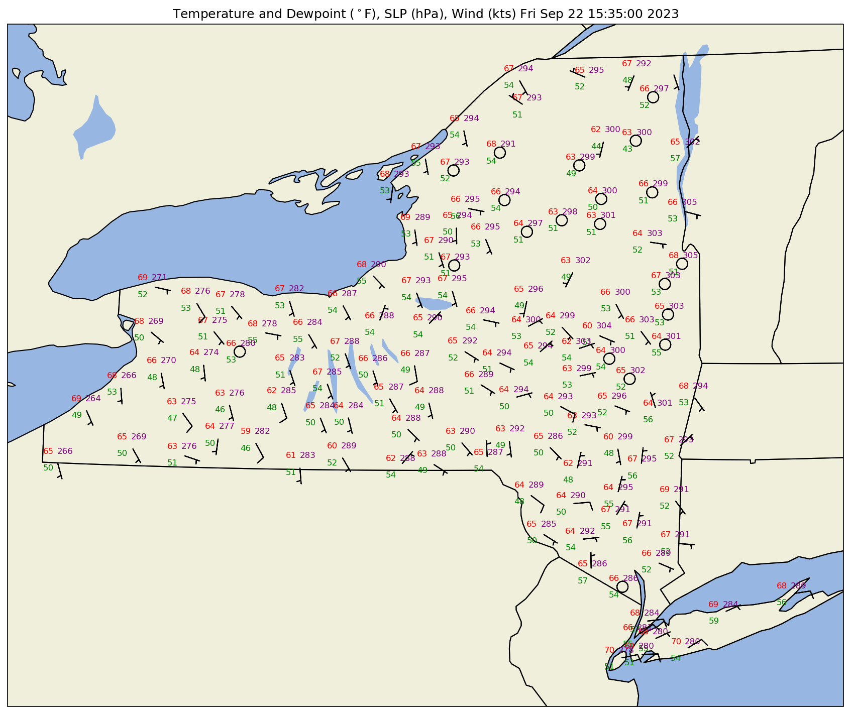
Create the map; first, add some cartographic features, and then plot the Mesonet observations at each station.
fig = plt.figure(figsize=(18,12),dpi=150) # Increase the dots per inch from default 100 to make plot easier to read
ax = fig.add_subplot(1,1,1,projection=proj)
ax.set_extent ([lonW,lonE,latS,latN])
# Choose the medium resolution of Natural Earth's cartographic features' shapefiles.
res = '50m'
# Set the default background color to that of a water body. This will be faster than plotting Cartopy's `OCEAN` feature's shapefile.
ax.set_facecolor(cfeature.COLORS['water'])
ax.add_feature (cfeature.LAND.with_scale(res))
ax.add_feature(cfeature.COASTLINE.with_scale(res))
ax.add_feature (cfeature.LAKES.with_scale(res))
ax.add_feature (cfeature.STATES.with_scale(res));

# Create a station plot pointing to an Axes to draw on as well as the location of points. Transform the station locations from lat-
stationplot = StationPlot(ax, lons, lats, transform=ccrs.PlateCarree(),
                          fontsize=8)

stationplot.plot_parameter('NW', tmpf, color='red')
stationplot.plot_parameter('SW', dwpf, color='green')

# A more complex example uses a custom formatter to control how the sea-level pressure
# values are plotted. This uses the standard trailing 3-digits of the pressure value
# in tenths of millibars.

stationplot.plot_parameter('NE', slp.values, color='purple', formatter=lambda v: format(10 * v, '.0f')[-3:])
stationplot.plot_barb(u, v,zorder=10)
ax.set_title ('Temperature and Dewpoint ($^\circ$F), SLP (hPa), Wind (kts) ' + timeStr);

# Save the figure to the current directory.
fig.savefig('nysm_sfcmap.png')