04_Xarray_Variables: More CFSR plotting¶

Overview¶

Select a date and access various CFSR Datasets
Subset the desired Datasets along their dimensions
Perform unit conversions
Create a well-labeled multi-parameter plot of gridded CFSR reanalysis data

Imports¶

import xarray as xr
import pandas as pd
import numpy as np
from datetime import datetime as dt
from metpy.units import units
import metpy.calc as mpcalc
import cartopy.crs as ccrs
import cartopy.feature as cfeature
import matplotlib.pyplot as plt

ERROR 1: PROJ: proj_create_from_database: Open of /knight/anaconda_aug22/envs/aug22_env/share/proj failed

Subset the desired `Dataset`s along their dimensions.¶

We will use the `sel` method on the latitude and longitude dimensions as well as time and isobaric surface.¶

# Areal extent
lonW = -100.
lonE = -60.
latS = 20.
latN = 50.
cLat, cLon = (latS + latN)/2, (lonW + lonE)/2

expand = 0.5
latRange = np.arange(latS,latN + expand, .5) # expand the data range a bit beyond the plot range
lonRange = np.arange(lonW,lonE + expand, .5) # Need to match longitude values to those of the coordinate variable

# Vertical level specificaton
plevel = 850
levelStr = f'{plevel}' # Use for the figure title


# Data variable selection; modify depending on what variables you are interested in

T = dsT['t'].sel(time=dateTime,lev=plevel,lat=latRange,lon=lonRange)
U = dsU['u'].sel(time=dateTime,lev=plevel,lat=latRange,lon=lonRange)
V = dsV['v'].sel(time=dateTime,lev=plevel,lat=latRange,lon=lonRange)

Output the level and time strings; we’ll use them to create the figure’s title.¶

levelStr, timeStr

('850', '1993-03-14 1200 UTC')

Let’s look at some of the attributes¶

T.units

'K'

U.units

'm s^-1'

V.units

'm s^-1'

Define our subsetted coordinate arrays of lat and lon. Pull them from any of the DataArrays. We’ll need to pass these into the contouring functions later on.¶

lats = T.lat
lons = T.lon

Perform unit conversions¶

We take the DataArrays and apply MetPy’s unit conversion method.¶

T = T.metpy.convert_units('degC')
U = U.metpy.convert_units('kts')
V = V.metpy.convert_units('kts')

Create a well-labeled multi-parameter plot of gridded CFSR reanalysis data¶

proj_map = ccrs.LambertConformal(central_longitude=cLon, central_latitude=cLat)
proj_data = ccrs.PlateCarree() # Our data is lat-lon; thus its native projection is Plate Carree.
res = '50m'

Now define the range of our contour values and a contour interval.¶

This of course will depend on the level, time, region, and variable.

T.min(), T.max()

(<xarray.DataArray 't' ()>
 <Quantity(-26.749984741210938, 'degree_Celsius')>
 Coordinates:
     time     datetime64[ns] 1993-03-14T12:00:00
     lev      float32 850.0,
 <xarray.DataArray 't' ()>
 <Quantity(16.95001220703125, 'degree_Celsius')>
 Coordinates:
     time     datetime64[ns] 1993-03-14T12:00:00
     lev      float32 850.0)

minTVal = -30
maxTVal = 22
cint = 2
Tcintervals = np.arange(minTVal, maxTVal, cint)
Tcintervals

array([-30, -28, -26, -24, -22, -20, -18, -16, -14, -12, -10,  -8,  -6,
        -4,  -2,   0,   2,   4,   6,   8,  10,  12,  14,  16,  18,  20])

Plot the map¶

In this example: filled contours of 850 hPa temperature and wind barbs.

Create a meaningful title string.

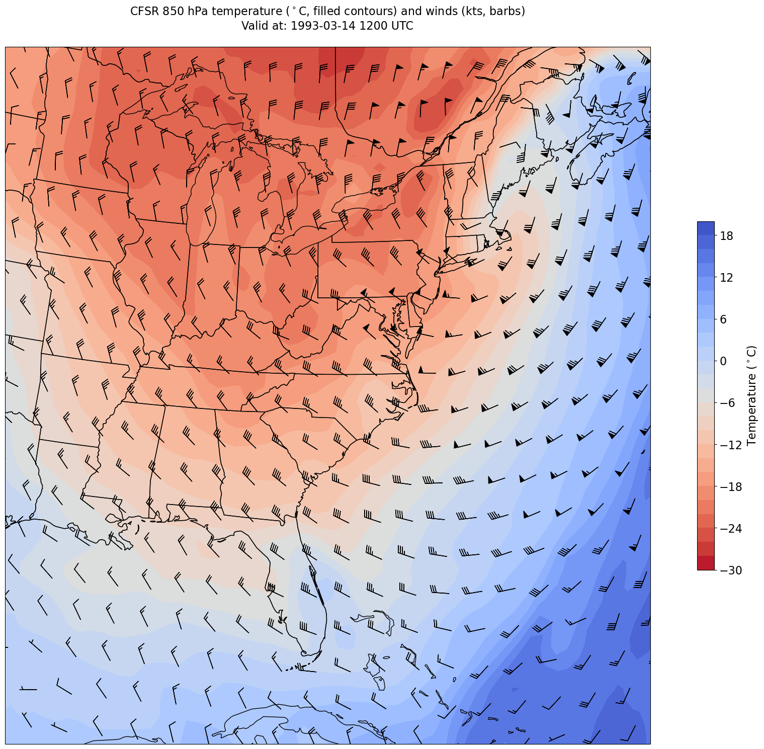
tl1 = f'CFSR {levelStr} hPa temperature ($^\circ$C, filled contours) and winds (kts, barbs)'
tl2 = f'Valid at: {timeStr}'
title_line = (tl1 + '\n' + tl2 + '\n') # concatenate the two strings and add return characters

constrainLat, constrainLon = (0.7, 6.5)

fig = plt.figure(figsize=(24,18)) # Increase size to adjust for the constrained lats/lons
ax = plt.subplot(1,1,1,projection=proj_map)
ax.set_extent ([lonW+constrainLon,lonE-constrainLon,latS+constrainLat,latN-constrainLat])
ax.add_feature(cfeature.COASTLINE.with_scale(res))
ax.add_feature(cfeature.STATES.with_scale(res))
CF = ax.contourf(lons,lats,T, levels=Tcintervals,transform=proj_data,cmap='coolwarm_r')
cbar = plt.colorbar(CF,shrink=0.5)
cbar.ax.tick_params(labelsize=16)
cbar.ax.set_ylabel("Temperature ($^\circ$C)",fontsize=16)

# Plotting wind barbs uses the ax.barbs method. Here, you can't pass in the DataArray directly; you can only pass in the array's values.
# Also need to sample (skip) a selected # of points to keep the plot readable.
skip = 3
ax.barbs(lons[::skip],lats[::skip],U[::skip,::skip].values, V[::skip,::skip].values, transform=proj_data)

title = plt.title(title_line,fontsize=16)

../../_images/04_Xarray_CFSR_Variables_34_0.png

ATM350 Spring 2023

04_Xarray_Variables: More CFSR plotting

Contents

04_Xarray_Variables: More CFSR plotting¶

Overview¶

Imports¶

Select a date and time, and access several CFSR Datasets¶

Create Xarray `Dataset` objects, each pointing to their respective NetCDF files in the `/cfsr/data` directory tree, using Xarray’s open_dataset method.¶

Let’s examine one of the Datasets.¶

Subset the desired `Dataset`s along their dimensions.¶

We will use the `sel` method on the latitude and longitude dimensions as well as time and isobaric surface.¶

Output the level and time strings; we’ll use them to create the figure’s title.¶

Let’s look at some of the attributes¶

Define our subsetted coordinate arrays of lat and lon. Pull them from any of the DataArrays. We’ll need to pass these into the contouring functions later on.¶

Perform unit conversions¶

We take the DataArrays and apply MetPy’s unit conversion method.¶

Create a well-labeled multi-parameter plot of gridded CFSR reanalysis data¶

Now define the range of our contour values and a contour interval.¶

Plot the map¶

Now, go back and try different variables, times, regional subsets, and levels!¶

ATM350 Spring 2023

04_Xarray_Variables: More CFSR plotting

Contents

04_Xarray_Variables: More CFSR plotting¶

Overview¶

Imports¶

Select a date and time, and access several CFSR Datasets¶

Create Xarray Dataset objects, each pointing to their respective NetCDF files in the /cfsr/data directory tree, using Xarray’s open_dataset method.¶

Let’s examine one of the Datasets.¶

Subset the desired Datasets along their dimensions.¶

We will use the sel method on the latitude and longitude dimensions as well as time and isobaric surface.¶

Output the level and time strings; we’ll use them to create the figure’s title.¶

Let’s look at some of the attributes¶

Define our subsetted coordinate arrays of lat and lon. Pull them from any of the DataArrays. We’ll need to pass these into the contouring functions later on.¶

Perform unit conversions¶

We take the DataArrays and apply MetPy’s unit conversion method.¶

Create a well-labeled multi-parameter plot of gridded CFSR reanalysis data¶

Now define the range of our contour values and a contour interval.¶

Plot the map¶

Now, go back and try different variables, times, regional subsets, and levels!¶

Create Xarray `Dataset` objects, each pointing to their respective NetCDF files in the `/cfsr/data` directory tree, using Xarray’s open_dataset method.¶

Subset the desired `Dataset`s along their dimensions.¶

We will use the `sel` method on the latitude and longitude dimensions as well as time and isobaric surface.¶