Cartopy 2: NYS Mesonet Data
Contents
Cartopy 2: NYS Mesonet Data
In this notebook, we’ll use Cartopy, Matplotlib, Datetime, and Pandas to visualize data from the New York State Mesonet, headquartered right here at UAlbany.
import matplotlib.pyplot as plt
import numpy as np
import pandas as pd
from cartopy import crs as ccrs
from cartopy import feature as cfeature
from datetime import datetime
ERROR 1: PROJ: proj_create_from_database: Open of /knight/anaconda_aug22/envs/aug22_env/share/proj failed
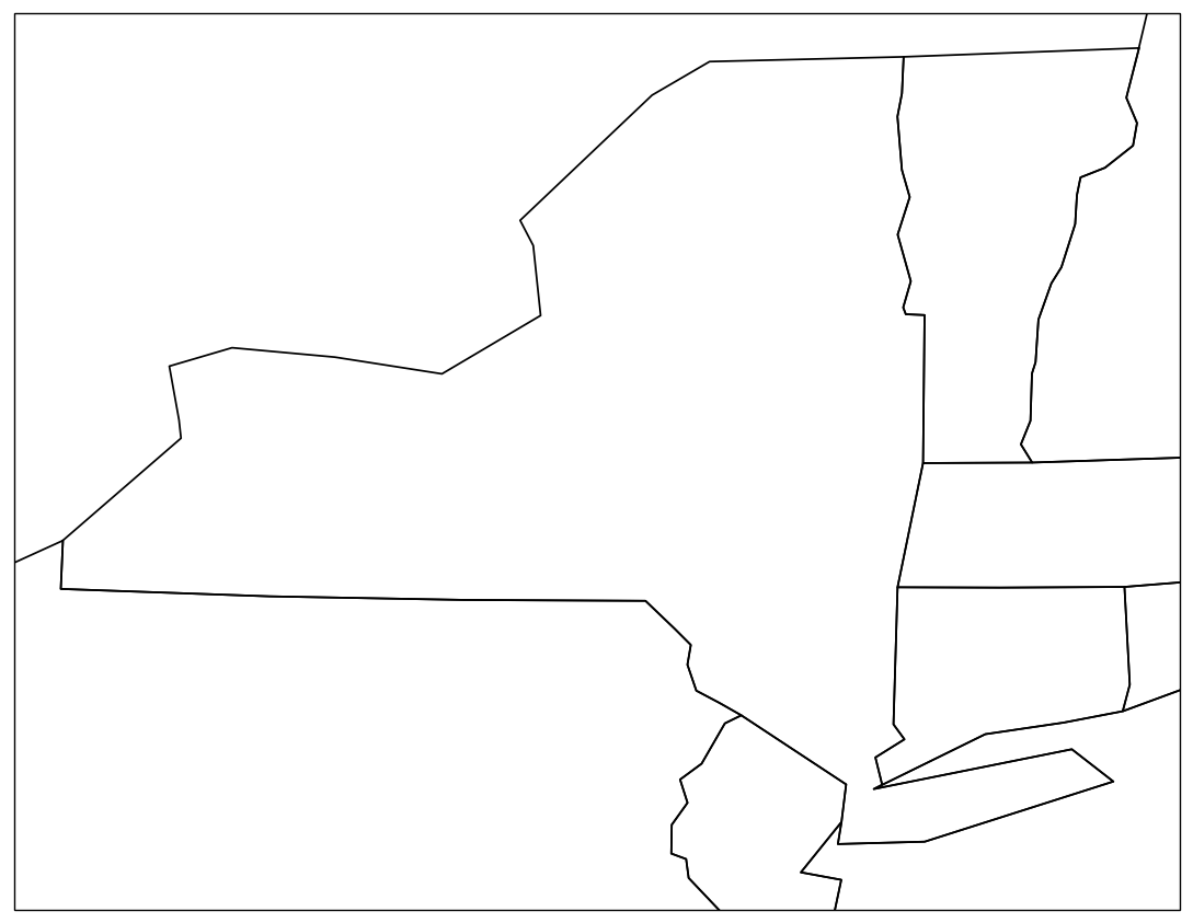
Create a regional map, centered over NYS, and add in some geographic features.
Be patient: this may take a minute or so to plot, depending on the resolution of the Natural Earth shapefile features you are adding!
Create the figure
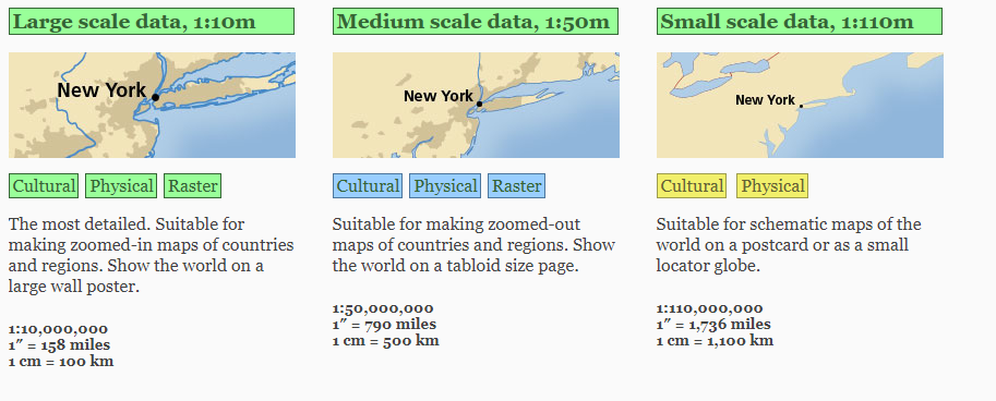
For a quick look, let’s just choose the coarsest (110,000,000:1) Natural Earth shapefiles set.
# Set the domain for defining the plot region.
latN = 45.2
latS = 40.2
lonW = -80.0
lonE = -71.5
cLat = (latN + latS)/2
cLon = (lonW + lonE )/2


proj = ccrs.LambertConformal(central_longitude=cLon, central_latitude=cLat)
#proj = ccrs.LambertConformal()
res = '110m' # Coarsest and quickest to display; other options are '10m' (slowest) and '50m'.

fig = plt.figure(figsize=(11,8.5),dpi=125)
ax = plt.subplot(1,1,1,projection=proj)
ax.set_extent ([lonW,lonE,latS,latN])
ax.add_feature(cfeature.COASTLINE.with_scale(res))
ax.add_feature (cfeature.STATES.with_scale(res));
Plot some data on the map. We’ll use Pandas to read in the file containing the most recent NYS Mesonet obs.
df = pd.read_csv('http://www.atmos.albany.edu/products/nysm/nysm_latest.csv')
View the first and last five lines of this DataFrame
df
| station | time | temp_2m [degC] | temp_9m [degC] | relative_humidity [percent] | precip_incremental [mm] | precip_local [mm] | precip_max_intensity [mm/min] | avg_wind_speed_prop [m/s] | max_wind_speed_prop [m/s] | ... | soil_temp_05cm [degC] | soil_temp_25cm [degC] | soil_temp_50cm [degC] | soil_moisture_05cm [m^3/m^3] | soil_moisture_25cm [m^3/m^3] | soil_moisture_50cm [m^3/m^3] | lat | lon | elevation | name | |
|---|---|---|---|---|---|---|---|---|---|---|---|---|---|---|---|---|---|---|---|---|---|
| 0 | ADDI | 2023-03-09 19:30:00 | 2.6 | 2.1 | 64.9 | 0.0 | 0.0 | 0.0 | 4.0 | 6.0 | ... | 0.8 | 1.8 | 2.5 | 0.59 | 0.44 | 0.43 | 42.040360 | -77.237260 | 507.6140 | Addison |
| 1 | ANDE | 2023-03-09 19:30:00 | -0.2 | -0.6 | 69.7 | 0.0 | 0.0 | 0.0 | 2.7 | 6.4 | ... | 1.4 | 2.0 | 2.7 | 0.29 | 0.18 | 0.17 | 42.182270 | -74.801390 | 518.2820 | Andes |
| 2 | BATA | 2023-03-09 19:30:00 | 0.2 | 0.3 | 66.2 | 0.0 | 0.0 | 0.0 | 2.8 | 3.6 | ... | 0.6 | 1.5 | 2.4 | 0.31 | 0.26 | 0.28 | 43.019940 | -78.135660 | 276.1200 | Batavia |
| 3 | BEAC | 2023-03-09 19:30:00 | 6.4 | 5.5 | 50.3 | 0.0 | 0.0 | 0.0 | 4.9 | 7.7 | ... | 4.8 | 3.9 | 4.0 | 0.35 | 0.41 | 0.39 | 41.528750 | -73.945270 | 90.1598 | Beacon |
| 4 | BELD | 2023-03-09 19:30:00 | -1.4 | -1.6 | 78.7 | 0.0 | 0.0 | 0.0 | 3.3 | 5.9 | ... | 1.1 | 1.5 | 2.2 | 0.46 | 0.48 | 0.41 | 42.223220 | -75.668520 | 470.3700 | Belden |
| ... | ... | ... | ... | ... | ... | ... | ... | ... | ... | ... | ... | ... | ... | ... | ... | ... | ... | ... | ... | ... | ... |
| 121 | WFMB | 2023-03-09 19:30:00 | -1.1 | -1.3 | 65.4 | 0.0 | 0.0 | 0.0 | 2.0 | 5.2 | ... | 0.5 | 1.1 | 1.6 | 0.25 | 0.21 | 0.23 | 44.393236 | -73.858829 | 614.5990 | Whiteface Mountain Base |
| 122 | WGAT | 2023-03-09 19:30:00 | -2.2 | -2.4 | 69.9 | 0.0 | 0.0 | 0.0 | 0.8 | 1.8 | ... | 0.2 | 0.6 | 1.1 | 0.14 | 0.26 | 0.08 | 43.532408 | -75.158597 | 442.9660 | Woodgate |
| 123 | WHIT | 2023-03-09 19:30:00 | 2.8 | 2.1 | 58.4 | 0.0 | 0.0 | 0.0 | 3.2 | 5.4 | ... | 0.5 | 1.1 | 2.2 | 0.61 | 0.52 | 0.50 | 43.485073 | -73.423071 | 36.5638 | Whitehall |
| 124 | WOLC | 2023-03-09 19:30:00 | -0.6 | -1.0 | 75.2 | 0.0 | 0.0 | 0.0 | 2.9 | 4.7 | ... | 0.4 | 0.8 | 1.4 | 0.24 | 0.04 | 0.12 | 43.228680 | -76.842610 | 121.2190 | Wolcott |
| 125 | YORK | 2023-03-09 19:30:00 | 2.5 | 1.5 | 65.9 | 0.0 | 0.0 | 0.0 | 2.0 | 4.6 | ... | 3.1 | 2.5 | 3.2 | 0.29 | 0.31 | 0.38 | 42.855040 | -77.847760 | 177.9420 | York |
126 rows × 34 columns
Examine the column names.
df.columns
Index(['station', 'time', 'temp_2m [degC]', 'temp_9m [degC]',
       'relative_humidity [percent]', 'precip_incremental [mm]',
       'precip_local [mm]', 'precip_max_intensity [mm/min]',
       'avg_wind_speed_prop [m/s]', 'max_wind_speed_prop [m/s]',
       'wind_speed_stddev_prop [m/s]', 'wind_direction_prop [degrees]',
       'wind_direction_stddev_prop [degrees]', 'avg_wind_speed_sonic [m/s]',
       'max_wind_speed_sonic [m/s]', 'wind_speed_stddev_sonic [m/s]',
       'wind_direction_sonic [degrees]',
       'wind_direction_stddev_sonic [degrees]', 'solar_insolation [W/m^2]',
       'station_pressure [mbar]', 'snow_depth [cm]', 'frozen_soil_05cm [bit]',
       'frozen_soil_25cm [bit]', 'frozen_soil_50cm [bit]',
       'soil_temp_05cm [degC]', 'soil_temp_25cm [degC]',
       'soil_temp_50cm [degC]', 'soil_moisture_05cm [m^3/m^3]',
       'soil_moisture_25cm [m^3/m^3]', 'soil_moisture_50cm [m^3/m^3]', 'lat',
       'lon', 'elevation', 'name'],
      dtype='object')
Create objects pointing to some columns of interest. In Pandas, we can refer to columns by using a “.” in addtion to “[]” in most circumstances, though not if a column name starts with a number, nor if there are spaces in the column name.
stid = df.station
lat = df.lat
lon = df.lon
tmp2 = df['temp_2m [degC]'] # Use brackets due to the presence of a space in the column name
tmp9 = df['temp_9m [degC]']
time = df.time
We will plot one of the variables on a map later on in this notebook. In case we want to go back later and pick a different variable to plot (e.g. 9 m temperature), let’s define a generic object name.
param = tmp9 # replace with tmp9, e.g., if you want to plot 9 m temperature
param
0      2.1
1     -0.6
2      0.3
3      5.5
4     -1.6
      ...
121   -1.3
122   -2.4
123    2.1
124   -1.0
125    1.5
Name: temp_9m [degC], Length: 126, dtype: float64
Let’s look at the time object.
time
0      2023-03-09 19:30:00
1      2023-03-09 19:30:00
2      2023-03-09 19:30:00
3      2023-03-09 19:30:00
4      2023-03-09 19:30:00
              ...
121    2023-03-09 19:30:00
122    2023-03-09 19:30:00
123    2023-03-09 19:30:00
124    2023-03-09 19:30:00
125    2023-03-09 19:30:00
Name: time, Length: 126, dtype: object
The times are the same for all stations, so let’s just pull out one of them, and then create some formatted datetime strings out of it.
timeString = time[0]
timeString
'2023-03-09 19:30:00'
The timeString above could make for a perfectly fine part of an informative title for a map, but let’s create a string of the form “Month Day, Year, HourMin UTC” (e.g., Mar 30, 2021, 0120 UTC )
First, make a datetime object from the string, using strptime with a format that matches that of the string.
timeObj = datetime.strptime(timeString,"%Y-%m-%d %H:%M:%S")
timeObj
datetime.datetime(2023, 3, 9, 19, 30)
Next, make a string object from the datetime object, using strftime with a format that matches what we want to use in the map’s title.
titleString = datetime.strftime(timeObj,"%B %d %Y, %H%M UTC")
titleString
'March 09 2023, 1930 UTC'
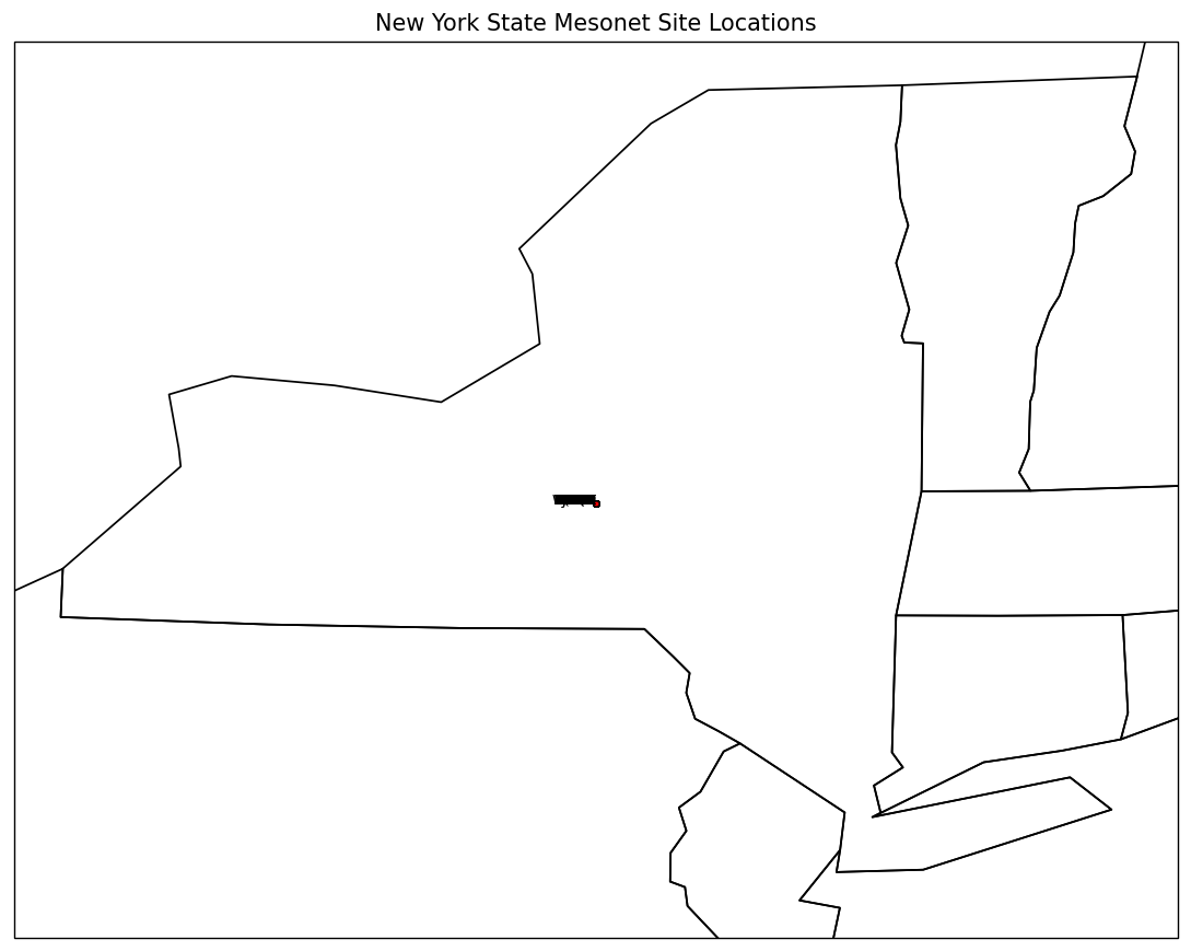
Create a scatterplot to show the locations of each NYS Mesonet site using Matplotlib’s scatter method. This method accepts an entire array of lon-lat values.
ax.set_title ('New York State Mesonet Site Locations')
ax.scatter(lon,lat,s=9,c='r',edgecolor='black',alpha=0.75,transform=ccrs.PlateCarree())
# Plot the figure, now with the sites plotted
fig
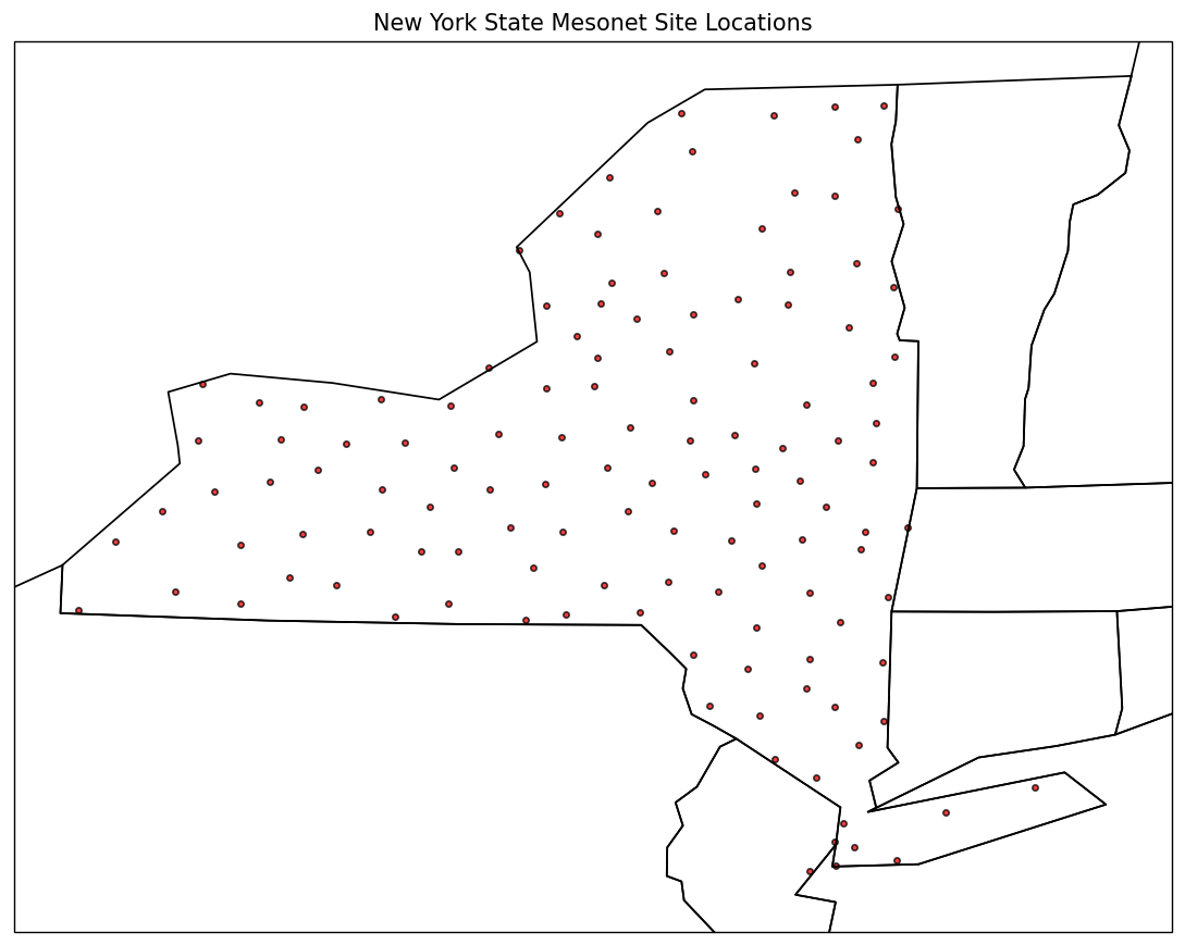
Did you notice the transform argument? Since we are plotting on a Lambert Conformal-projected map, which uses a Cartesian x-y coordinate system where each point is equally separated in meters, we need to convert, or transform, the lat-lon coordinates into their equivalent coordinates in our chosen projection. We use the transform argument, and assign its value to the coordinate system that our lat-lon array is derived from.
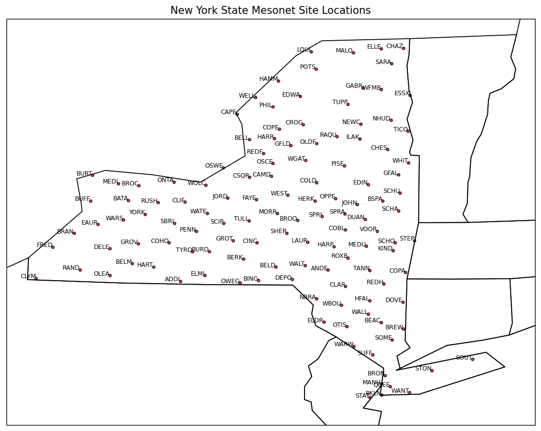
Next, plot the site IDs, using Matplotlib’s text method. This method only accepts a single value for its x and y coordinates, so we need to loop over all the values in the arrays.
Recall that in a Python list, one can use the enumerate function to set a numerical value to be used as a counter. We can use the same technique on a Pandas series object:
for count, site in enumerate(stid):
    print (count, site)
0 ADDI
1 ANDE
2 BATA
3 BEAC
4 BELD
5 BELL
6 BELM
7 BERK
8 BING
9 BKLN
10 BRAN
11 BREW
12 BROC
13 BRON
14 BROO
15 BSPA
16 BUFF
17 BURD
18 BURT
19 CAMD
20 CAPE
21 CHAZ
22 CHES
23 CINC
24 CLAR
25 CLIF
26 CLYM
27 COBL
28 COHO
29 COLD
30 COPA
31 COPE
32 CROG
33 CSQR
34 DELE
35 DEPO
36 DOVE
37 DUAN
38 EAUR
39 EDIN
40 EDWA
41 ELDR
42 ELLE
43 ELMI
44 ESSX
45 FAYE
46 FRED
47 GABR
48 GFAL
49 GFLD
50 GROT
51 GROV
52 HAMM
53 HARP
54 HARR
55 HART
56 HERK
57 HFAL
58 ILAK
59 JOHN
60 JORD
61 KIND
62 LAUR
63 LOUI
64 MALO
65 MANH
66 MEDI
67 MEDU
68 MORR
69 NBRA
70 NEWC
71 NHUD
72 OLDF
73 OLEA
74 ONTA
75 OPPE
76 OSCE
77 OSWE
78 OTIS
79 OWEG
80 PENN
81 PHIL
82 PISE
83 POTS
84 QUEE
85 RAND
86 RAQU
87 REDF
88 REDH
89 ROXB
90 RUSH
91 SARA
92 SBRI
93 SCHA
94 SCHO
95 SCHU
96 SCIP
97 SHER
98 SOME
99 SOUT
100 SPRA
101 SPRI
102 STAT
103 STEP
104 STON
105 SUFF
106 TANN
107 TICO
108 TULL
109 TUPP
110 TYRO
111 VOOR
112 WALL
113 WALT
114 WANT
115 WARS
116 WARW
117 WATE
118 WBOU
119 WELL
120 WEST
121 WFMB
122 WGAT
123 WHIT
124 WOLC
125 YORK
We’ll repeat the enumeration below; instead of printing out the counter value and its associated list element name, we’ll pass them in directly to Matplotlib’s ax.text function:
for count, site in enumerate(stid):
    ax.text(lon[count],lat[count],site,horizontalalignment='right',transform=ccrs.PlateCarree(),fontsize=7)
fig
Now, let’s attempt to plot the site locations again, but this time we’ll omit the transform argument in ax.scatter and ax.text.
fig = plt.figure(figsize=(11,8.5),dpi=125)
ax = plt.subplot(1,1,1,projection=proj)
ax.set_extent ([lonW,lonE,latS,latN])
ax.add_feature(cfeature.COASTLINE.with_scale(res))
ax.add_feature (cfeature.STATES.with_scale(res))
ax.set_title ('New York State Mesonet Site Locations')
ax.scatter(lon,lat,s=9,c='r',edgecolor='black',alpha=0.75)
for count, site in enumerate(stid):
    ax.text(lon[count],lat[count],site,horizontalalignment='right',fontsize=7)
What do you think happened here?
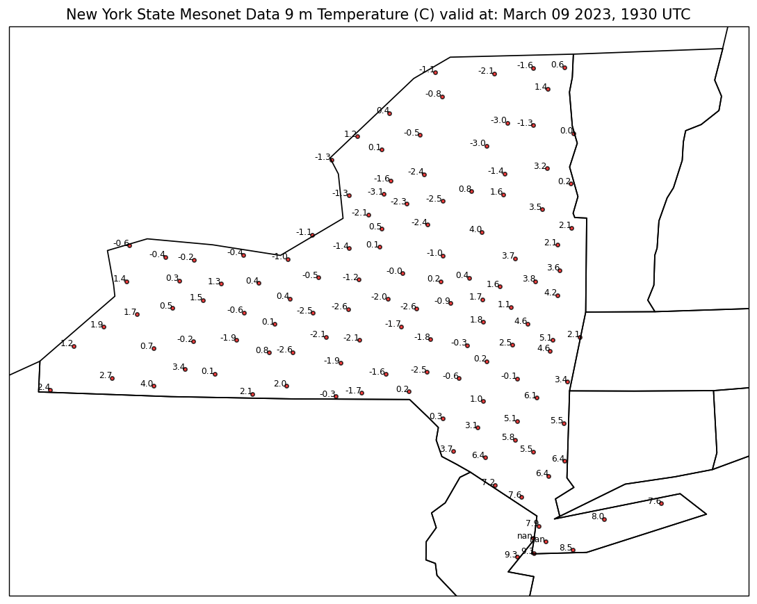
Exercise
Create a new figure which plots the current 2m temperature at the NYSM sites. Include the current date/time to the title.
fig = plt.figure(figsize=(11,8.5),dpi=125)
ax = plt.subplot(1,1,1,projection=proj)
ax.set_extent ([lonW,lonE,latS,latN])
ax.add_feature(cfeature.COASTLINE.with_scale(res))
ax.add_feature (cfeature.STATES.with_scale(res))
ax.set_title ('New York State Mesonet Data 9 m Temperature (C) valid at: ' + titleString)
ax.scatter(lon,lat,s=9,c='r',edgecolor='black',alpha=0.75,transform=ccrs.PlateCarree())
for count, value in enumerate(param):
    ax.text(lon[count],lat[count],value,horizontalalignment='right',fontsize=7,transform=ccrs.PlateCarree())
# %load '/spare11/atm350/common/mar07/mar07.py'
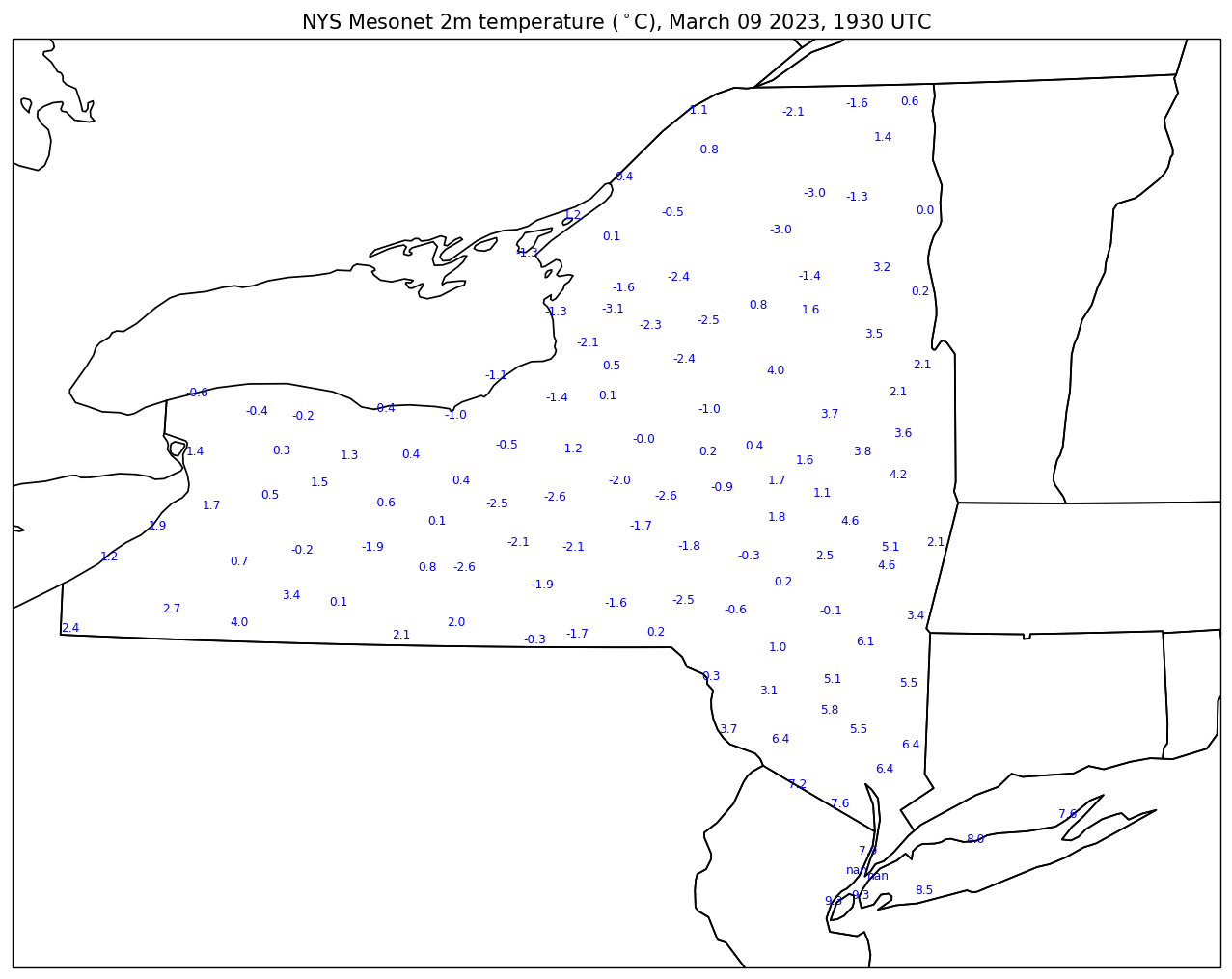
proj = ccrs.LambertConformal(central_longitude=cLon, central_latitude=cLat)
res = '50m' # Use the medium-resolution shapefiles
fig = plt.figure(figsize=(15,10),dpi=125)
ax = plt.subplot(1,1,1,projection=proj)
ax.set_extent ([lonW,lonE,latS,latN])
ax.set_title("NYS Mesonet 2m temperature ($^\circ$C), " + titleString)
ax.add_feature(cfeature.COASTLINE.with_scale(res))
ax.add_feature (cfeature.STATES.with_scale(res));
for count, value in enumerate(param):
ax.text(lon[count],lat[count],value,horizontalalignment='right',transform=ccrs.PlateCarree(),fontsize=7,color='blue')